International Journal of Emerging Technology and Advanced Engineering
Website: www.ijetae.com (ISSN 2250-2459, ISO 9001:2008 Certified Journal, Volume 7, Issue 9, September 2017)
381
Solving Singularly Perturbed Differential-Difference Equations
using Special Finite Difference Method
V. Vidyasagar
1,
Madhu Latha K
1, B. Ravindra Reddy
21Department of Mathematics, Kamala Institute Of Technology & Science, Huzurabad, JNTUH, India 2Department of Mathematics, JNTUH College of Engineering, Hyderabad-500085, India
Abstract: In this paper, we present a special finite difference method to solve singularly perturbed differential-difference equations with layer behavior. In this special second order method, we use a second order finite difference approximation for second order derivative, a modified second order upwind finite difference approximation for first order
derivative and a second order average difference
approximation for y. The Thomas algorithm is used to solve
the tridiagonal system. To validate the computational efficiency of the method, a few model examples have been
solved for different values of perturbation parameter, delay
parameter , advanced parameter . We have presented
maximum absolute errors for the standard examples chosen from the literature.
Keywords— boundary layer , central differences ,differential-difference equations, finite difference.
I. INTRODUCTION
The highest order derivative is multiplied by a perturbation parameter is known as the singular perturbation problem. A differential equation in which the highest derivative is multiplied by a small positive parameter and containing at least one shift term(delay or advance) is known as singularly perturbed differential-difference equation. Prasad and Reddy [1] developed differential quadrature method for finding the numerical solution of boundary-value problems for a singularly perturbed differential-difference equation of mixed type. In the current reviews led by Kadalbajoo and Sharma [2],[3], Kadalbajoo and Ramesh [4] and Kadalbajoo and Kumar [5],[6], the terms negative or left shift and positive or right shift have been utilized for delay and advance respectively. The differential-difference equation plays an essential role in the mathematical modeling of various practical phenomena in the biosciences and control theory. Any system including a feedback control will quite include often time delays. These arise because a finite time is required to sense information and after that respond to it. For a point by point examination on differential-difference equation, one may refer to Bellen and Zennaro [7], Driver [8], Bellman and Cooke [9] books and high level monographs.
In El’sgol’ts [10], similar boundary value problems with solutions that show quick oscillations are considered. Kadalbajoo and Sharma [2],[3], Kadalbajoo and Ramesh [4] and Kadalbajoo and Kumar [5],[6] started a broad numerical work for solving singularly perturbed delay differential equations based on finite difference scheme, fitted mesh and B-spline method, piecewise uniform mesh. Lange and Miura [11],[12] gave asymptotic approaches in the study of class of boundary value problems for linear second order differential difference equations in which the highest order derivative is multiplied by small parameter. They have also additionally talked about the impact of small shifts on the oscillatory solution of the problem.Duressa et al. and Sirisha L et al. [13],[14] exhibited numerical methods to approximate the solution of boundary value problems for SPDDEs with delay as well as advance.
II. DESCRIPTION OF THE METHOD
Consider singularly perturbed differential-difference equation with delay as well as advance parameters of the form:
) ( ) ( ) ( ) ( ) ( ) ( ) ( ) ( ) ( )
(x axy x bxyx cxyx d xyx f x
y
(1)
) 1 , 0 (
x subject to the interval and boundary conditions
0 on
), ( )
(x x x
y (2)
( ), on 1 1 )
(x x x
y (3)
where
) ( and ) ( ), ( ), ( ), ( ),
(x b x c x d x x x
a are bounded and
continuously differentiable functions on (0, 1), 01 is the singular perturbation parameter; and 0O()
and 0O() are the delay and the advance parameters respectively. In general, the solution of Eqs. (1)-(3) exhibits the boundary layer behavior at one end of the interval [0,1] depending upon the sign.
International Journal of Emerging Technology and Advanced Engineering
Website: www.ijetae.com (ISSN 2250-2459, ISO 9001:2008 Certified Journal, Volume 7, Issue 9, September 2017)
382 ) ( ) ( )
(x y x y x
y (4)
) ( ) ( )
(x y x y x
y (5)
Using Eq. (4) and Eq. (5) in Eq. (1) we get an asymptotically equivalent singularly perturbed boundary value problem of the form:
) ( ) ( ) ( ) ( ) ( )
(x p x y x q x y x f x
y
(6)
0 ) 0 ( ) 0 (
y (7)
1 ) 1 ( ) 1 (
y
(8)
Where ( ) ) ( ) ( )
(x ax d x bx
p and (9)
) ( ) ( ) ( )
(x b x c x d x
q (10)
The transition from Eq.(1) to Eq.(6) is admitted, because of the condition that01 and 01 are sufficiently small. This substitution is significant from the computational point of view. Further details on the validity of this transition is found in El’sgol’ts and Norkin[15]. Thus, the solution of Eq.(6) will give a good approximation to the solution of Eq.(1). Further, we assume that
0 ) ( ) ( ) ( )
(x a x d x b x M
p
0 ) ( ) ( ) ( )
(x b x c x d x
q
Throughout the interval [0, 1], where M is some positive constant. Under these assumption, Eq.(6) has a unique solution y(x) which shows a boundary layer of width
) (
O on the left side (x = 0) of the underlying interval. Divide the interval [0, 1] into N equal parts with constant mesh length h. Let 0=
x
1,
x
2,...
x
N=1 be themesh points. Then we have
x
i
ih
:
i
0, 1, 2, ……,N.At
x
x
i the equation (6) becomes)
( i i i i i
i x py qy f
y
III. LEFT –END BOUNDARY LAYER PROBLEM
We assume that q(x) ≤ 0, p(x) ≥ M >0 throughout the interval [0, 1], where M is some positive constant.
Under these assumptions, Eq.(6) has a unique solution
y(x) which in general, displays a boundary layer of width O() at x = 0 for small values of .
We extended the idea given by Van Veldhuizen[16] to the boundary value problem Eq.(6) by considering the special second difference method for the equation Eq.(6) as follows:
2
2
2
1 1i 1 2 1 1 i i i i i i i i i i
f
y
y
q
y
h
h
y
y
p
h
y
y
y
2
2
2
1 1 i i 1 2 1 1 i i i i i i i i i i i i if
y
y
q
y
q
y
p
f
h
h
y
y
p
h
y
y
y
(11) 2 / 1 1 1 i 2 / 1 2 / 1 1 2 1 12
2
2
2
2
i i i i i i i i i i i i i i i i if
h
p
f
y
y
q
y
h
q
p
y
h
p
p
h
y
y
p
h
y
y
y
(12) Substitutingh
y
y
y
i
i1
i in the above equation andsimplifying, we get
2 / 1 1 i 2 / 1 2 2 / 1 2 / 1 2 1 i 2
2
2
2
2
2
2
2
i i i i i i i i i i i i i if
h
p
f
y
q
p
p
h
p
h
y
h
q
p
p
p
h
p
h
y
q
h
(13)From this we can get a three term recurrence relation of the form 1 ,..., 2 , 1 i ; 1
1
Fy Gy H N
y
International Journal of Emerging Technology and Advanced Engineering
Website: www.ijetae.com (ISSN 2250-2459, ISO 9001:2008 Certified Journal, Volume 7, Issue 9, September 2017)
383 Where 2 / 1 i 2 / 1 2 2 / 1 2 / 1 2 i 2 2 2 2 2 2 2 2 i i i i i i i i i i i i i i i f h p f H q p p h p h G h q p p p h p h F q h E
We solve the system of equations (14) by using the Thomas algorithm.
IV. RIGHT –END BOUNDARY LAYER PROBLEM
Now we assume that p(x),q(x) and f(x) are sufficiently continuously differentiable functions in [0, 1] and q(x) ≤ 0, p(x) ≤ M < 0 throughout the interval [0, 1], where M is
some negative constant. Under these assumptions, Eq.(6) has a unique solution y(x) which in general, displays a boundary layer of width O() at x = 1 for small values of
.
For this right–end boundary layer problems weconsider the special second order finite difference method as:
2
2
2
1 1i 1 2 1 1 i i i i i i i i i
i
h
y
q
y
y
f
h
y
y
p
h
y
y
y
(15)2
2
2
1 1 i i 1 2 1 1 i i i i i i i i i i i i if
y
y
q
y
q
y
p
f
h
h
y
y
p
h
y
y
y
(16) 2 / 1 1 i 2 2 / 1 2 / 1 2 1 2 / 1 22
-
2
2
2
2
2
2
i i i i i i i i i i i i i i if
h
p
f
y
q
h
y
h
q
p
p
p
h
p
h
y
q
p
p
h
p
h
(17)From this we can get a three term recurrence relation of the form 1 ,..., 2 , 1 i ; 1
1
Fy Gy H N
y
Ei i i i i i i (18)
where 2 / 1 i 2 2 / 1 2 / 1 2 2 / 1 2 2 2 2 2 2 2 2 i i i i i i i i i i i i i i i i f h p f H q h G h q p p p h p h F q p p h p h E
We solve the tridiagonal system of equations (18) by using the Thomas algorithm.
V. NUMERICAL EXAMPLES
To demonstrate the applicability of the method we have applied it to three linear singular perturbation problems with left-end boundary layer and three linear singular perturbation problems with right-end boundary layer. These examples have been chosen because they have been widely discussed in literature. The numerical solutions are compared with the exact solutions. The exact solution of singularly perturbed differential-difference equation:
) ( ) ( ) ( ) ( ) ( ) ( ) ( ) ( ) ( )
(x axy x bxyx cx yx d xyx f x
y
) 1 , 0 (
x and subject to the interval and boundary
conditions 1 1 on ), ( ) ( 0 on ), ( ) ( x x x y x x x y
with constant coefficients i.e,
) ( and ) ( , ) ( , ) ( , ) ( , ) ( , ) ( x x f x f d x d c x c b x b a x a
the exact solution is given by
3 2
1 /
)
(x ce 1 c e 2 f c
y mx mx
International Journal of Emerging Technology and Advanced Engineering
Website: www.ijetae.com (ISSN 2250-2459, ISO 9001:2008 Certified Journal, Volume 7, Issue 9, September 2017)
384
d c b
c e e
c f e c f c
c e e
c f e c f c
m m
m m m
m
3
3 3 3
2
3 3 3
1
c
, )
(
) (
, )
(
) (
2 1
2 2 1
2
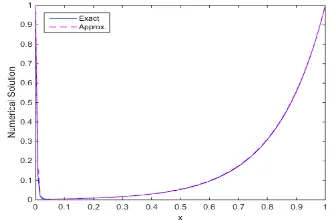
Example 1: Consider the singularly perturbed differential-difference equation with left end boundary layer:
1 ) ( , 1 ) ( , 0 ) ( 3 ) ( 2 ) ( )
(
x y x y x y x x x
y
The numerical results are presented in Tables I(a) and I(b) and Figure 1
Example 2:Consider the singularly perturbed differential-difference equation with left end boundary layer:
1 ) ( , 1 ) ( , 0 ) ( 2 ) ( 3 ) ( )
(
x y x y x y x x x
y
The numerical results are presented in Tables II(a) and II(b) and Figure 2
Example 3: Consider the singularly perturbed differential-difference equation with left end boundary layer:
1 ) ( , 1 ) ( , 0 ) ( ) ( 5 ) ( 2 ) ( )
(
x y x y x yx yx x x
y
The numerical results are presented in Tables III(a) and III(b) and Figure 3
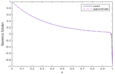
Example 4: Consider the singularly perturbed differential-difference equation with right end boundary layer:
1 ) ( , 1 ) ( , 0 ) ( ) ( 2 ) ( )
(
x y x y x y x x x
y
The numerical results are presented in Tables IV(a) and IV(b) and Figure 4
Example 5: Consider the singularly perturbed differential-difference equation with right end boundary layer:
1 ) ( , 1 ) ( , 0 ) ( 2 ) ( ) ( )
(
x y x yx yx x x
y
The numerical results are presented in Tables V(a) and V(b) and Figure 5
Example 6: Consider the singularly perturbed differential-difference equation with right end boundary layer:
1 ) ( , 1 ) ( , 0 ) ( 2 ) ( ) ( 2 ) ( )
(
x y x yx yx yx x x
y
[image:4.612.354.526.191.303.2]The numerical results are presented in Tables VI(a) and VI(b) and Figure 6
[image:4.612.350.531.340.436.2]Figure 1. Numerical solution of Example 1 with h27, 28
Figure 2. Numerical solution of Example 2 with h27, 28
[image:4.612.357.525.473.583.2]International Journal of Emerging Technology and Advanced Engineering
Website: www.ijetae.com (ISSN 2250-2459, ISO 9001:2008 Certified Journal, Volume 7, Issue 9, September 2017)
[image:5.612.347.533.146.266.2] [image:5.612.75.251.149.308.2]385 Figure 4. Numerical solution of Example 4 with h27, 28
Figure 5. Numerical solution of Example 5 with h27, 28
Figure 6. Numerical solution of Example 6 with h27, 28
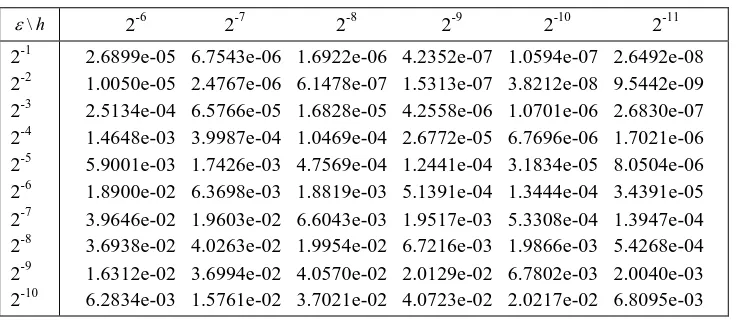
Table I (a)
The absolute maximum errors in solution of Example 1 for 0.1 and 0.1
h
\
2-6 2
-7
2-8 2-9 2-10 2-11
2-1 2-2 2-3 2-4 2-5 2-6 2-7 2-8 2-9 2-10
[image:5.612.64.270.345.474.2] [image:5.612.123.488.543.702.2]International Journal of Emerging Technology and Advanced Engineering
Website: www.ijetae.com (ISSN 2250-2459, ISO 9001:2008 Certified Journal, Volume 7, Issue 9, September 2017)
386 Table I (b)
The absolute maximum errors in solution of Example 1 for 0.5 and 0.5
h
\
2-6 2
-7
2-8 2-9 2-10 2-11
2-1 2-2 2-3 2-4 2-5 2-6 2-7 2-8 2-9 2-10
2.6899e-05 6.7543e-06 1.6922e-06 4.2352e-07 1.0594e-07 2.6492e-08 1.0050e-05 2.4767e-06 6.1478e-07 1.5313e-07 3.8212e-08 9.5442e-09 2.5134e-04 6.5766e-05 1.6828e-05 4.2558e-06 1.0701e-06 2.6830e-07 1.4648e-03 3.9987e-04 1.0469e-04 2.6772e-05 6.7696e-06 1.7021e-06 5.9001e-03 1.7426e-03 4.7569e-04 1.2441e-04 3.1834e-05 8.0504e-06 1.8900e-02 6.3698e-03 1.8819e-03 5.1391e-04 1.3444e-04 3.4391e-05 3.9646e-02 1.9603e-02 6.6043e-03 1.9517e-03 5.3308e-04 1.3947e-04 3.6938e-02 4.0263e-02 1.9954e-02 6.7216e-03 1.9866e-03 5.4268e-04 1.6312e-02 3.6994e-02 4.0570e-02 2.0129e-02 6.7802e-03 2.0040e-03 6.2834e-03 1.5761e-02 3.7021e-02 4.0723e-02 2.0217e-02 6.8095e-03
Table II (a)
The absolute maximum errors in solution of Example 2 for 0.1 and 0.1
h
\
2-6 2-7 2-8 2-9 2-10 2-11
2-1 2-2 2-3 2-4 2-5 2-6 2-7 2-8 2-9 2-10
1.4358e-06 3.4492e-07 8.4487e-08 2.0904e-08 5.1736e-09 1.3176e-09 5.9152e-05 1.5242e-05 3.8684e-06 9.7443e-07 2.4455e-07 6.1206e-08 3.7770e-04 9.9311e-05 2.5476e-05 6.4515e-06 1.6233e-06 4.0719e-07 1.6783e-03 4.6050e-04 1.2076e-04 3.0930e-05 7.8283e-06 1.9691e-06 6.2124e-03 1.8440e-03 5.0484e-04 1.3224e-04 3.3852e-05 8.5644e-06 1.9272e-02 6.5194e-03 1.9310e-03 5.2811e-04 1.3826e-04 3.5384e-05 3.9636e-02 1.9782e-02 6.6774e-03 1.9758e-03 5.4007e-04 1.4136e-04 3.6719e-02 4.0250e-02 2.0042e-02 6.7576e-03 1.9985e-03 5.4615e-04 1.6235e-02 3.6881e-02 4.0562e-02 2.0173e-02 6.7981e-03 2.0100e-03 6.2700e-03 1.5722e-02 3.6963e-02 4.0718e-02 2.0238e-02 6.8184e-03
Table II (b)
The absolute maximum errors in solution of Example 2 for 0.5 and 0.5
h
\
2-6 2-7 2-8 2-9 2-10 2-11
2-1 2-2 2-3 2-4 2-5 2-6 2-7 2-8 2-9 2-10
[image:6.612.124.495.164.325.2] [image:6.612.121.493.359.514.2] [image:6.612.124.493.548.703.2]International Journal of Emerging Technology and Advanced Engineering
Website: www.ijetae.com (ISSN 2250-2459, ISO 9001:2008 Certified Journal, Volume 7, Issue 9, September 2017)
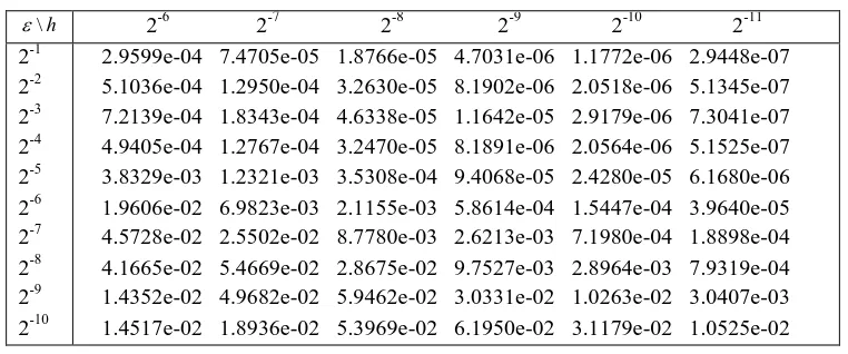
387 Table III (a)
The absolute maximum errors in solution of Example 3 for 0.1 and 0.1
h
\
2-6 2
-7
2-8 2-9 2-10 2-11 2-1
2-2 2-3 2-4 2-5 2-6 2-7 2-8 2-9 2-10
2.9599e-04 7.4705e-05 1.8766e-05 4.7031e-06 1.1772e-06 2.9448e-07 5.1036e-04 1.2950e-04 3.2630e-05 8.1902e-06 2.0518e-06 5.1345e-07 7.2139e-04 1.8343e-04 4.6338e-05 1.1642e-05 2.9179e-06 7.3041e-07 4.9405e-04 1.2767e-04 3.2470e-05 8.1891e-06 2.0564e-06 5.1525e-07 3.8329e-03 1.2321e-03 3.5308e-04 9.4068e-05 2.4280e-05 6.1680e-06 1.9606e-02 6.9823e-03 2.1155e-03 5.8614e-04 1.5447e-04 3.9640e-05 4.5728e-02 2.5502e-02 8.7780e-03 2.6213e-03 7.1980e-04 1.8898e-04 4.1665e-02 5.4669e-02 2.8675e-02 9.7527e-03 2.8964e-03 7.9319e-04 1.4352e-02 4.9682e-02 5.9462e-02 3.0331e-02 1.0263e-02 3.0407e-03 1.4517e-02 1.8936e-02 5.3969e-02 6.1950e-02 3.1179e-02 1.0525e-02
Table III (b)
The absolute maximum errors in solution of Example 3 for0.5 and 0.5
h
\
2-6 2-7 2-8 2-9 2-10 2-11
2-1 2-2 2-3 2-4 2-5 2-6 2-7 2-8 2-9 2-10
2.1761e-04 5.5060e-05 1.3851e-05 3.4737e-06 8.6982e-07 2.1763e-07 3.9292e-04 9.9729e-05 2.5143e-05 6.3115e-06 1.5812e-06 3.9571e-07 5.0782e-04 1.2760e-04 3.2029e-05 8.0208e-06 2.0070e-06 5.0199e-07 5.9098e-04 1.5409e-04 3.9368e-05 9.9522e-06 2.5021e-06 6.2729e-07 4.4906e-03 1.4474e-03 4.1278e-04 1.0994e-04 2.8394e-05 7.2128e-06 2.0506e-02 7.3173e-03 2.2210e-03 6.1738e-04 1.6263e-04 4.1770e-05 4.6137e-02 2.5951e-02 8.9471e-03 2.6750e-03 7.3504e-04 1.9316e-04 4.1575e-02 5.4844e-02 2.8898e-02 9.8375e-03 2.9234e-03 8.0088e-04 1.4307e-02 4.9608e-02 5.9541e-02 3.0442e-02 1.0306e-02 3.0542e-03 1.4503e-02 1.8902e-02 5.3924e-02 6.1988e-02 3.1234e-02 1.0547e-02
Table IV (a)
The absolute maximum errors in solution of Example 4 for 0.1 and 0.1
h
\
2-6 2-7 2-8 2-9 2-10 2-11
2-1 2-2 2-3 2-4 2-5 2-6 2-7 2-8 2-9
[image:7.612.116.497.163.322.2] [image:7.612.118.500.356.511.2] [image:7.612.118.497.549.690.2]International Journal of Emerging Technology and Advanced Engineering
Website: www.ijetae.com (ISSN 2250-2459, ISO 9001:2008 Certified Journal, Volume 7, Issue 9, September 2017)
388 Table IV (b)
The absolute maximum errors in solution of Example 4 for0.5 and 0.5
h
\
2-6 2
-7
2-8 2-9 2-10 2-11 2-1
2-2 2-3 2-4 2-5 2-6 2-7 2-8 2-9
3.5393e-05 8.8772e-06 2.2231e-06 5.5625e-07 1.3912e-07 3.4788e-08 4.8202e-05 1.1992e-05 2.9907e-06 7.4677e-07 1.8658e-07 4.6629e-08 3.6119e-04 9.5705e-05 2.4618e-05 6.2435e-06 1.5721e-06 3.9443e-07 2.6896e-03 7.3827e-04 1.9360e-04 4.9605e-05 1.2553e-05 3.1573e-06 1.1773e-02 3.4931e-03 9.5580e-04 2.5028e-04 6.4055e-05 1.6205e-05 3.9180e-02 1.3253e-02 3.9236e-03 1.0726e-03 2.8075e-04 7.1840e-05 8.2249e-02 4.1536e-02 1.4018e-02 4.1464e-03 1.1331e-03 2.9655e-04 7.4414e-02 8.5333e-02 4.2731e-02 1.4406e-02 4.2597e-03 1.1640e-03 2.8268e-02 7.7276e-02 8.6888e-02 4.3332e-02 1.4602e-02 4.3169e-03
Table V (a)
The absolute maximum errors in solution of Example 5 for 0.1 and 0.1
h
\
2-6 2
-7
2-8 2-9 2-10 2-11 2-1
2-2 2-3 2-4 2-5 2-6 2-7 2-8 2-9
1.8379e-05 4.5586e-06 1.1351e-06 2.8321e-07 7.0744e-08 1.7664e-08 7.9967e-05 2.0941e-05 5.3584e-06 1.3551e-06 3.4071e-07 8.5443e-08 6.8869e-04 1.8247e-04 4.6992e-05 1.1921e-05 3.0022e-06 7.5328e-07 3.3206e-03 9.1941e-04 2.4188e-04 6.2060e-05 1.5716e-05 3.9545e-06 1.2825e-02 3.8238e-03 1.0493e-03 2.7547e-04 7.0559e-05 1.7859e-05 4.0614e-02 1.3789e-02 4.0925e-03 1.1204e-03 2.9351e-04 7.5155e-05 8.2892e-02 4.2257e-02 1.4288e-02 4.2317e-03 1.1573e-03 3.0300e-04 7.4254e-02 8.5648e-02 4.3092e-02 1.4542e-02 4.3026e-03 1.1761e-03 2.8173e-02 7.7189e-02 8.7044e-02 4.3513e-02 1.4670e-02 4.3384e-03
Table V (b)
The absolute maximum errors in solution of Example 5 for0.5 and 0.5
h
\
2-6 2-7 2-8 2-9 2-10 2-11
2-1 2-2 2-3 2-4 2-5 2-6 2-7 2-8 2-9
[image:8.612.118.498.162.305.2] [image:8.612.122.496.340.482.2] [image:8.612.118.496.520.660.2]International Journal of Emerging Technology and Advanced Engineering
Website: www.ijetae.com (ISSN 2250-2459, ISO 9001:2008 Certified Journal, Volume 7, Issue 9, September 2017)
389 Table VI (a)
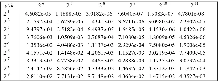
The absolute maximum errors in solution of Example 6 for 0.1 and 0.1
h
\
2-6 2
-7
2-8 2-9 2-10 2-11 2-1
2-2 2-3 2-4 2-5 2-6 2-7 2-8 2-9
1.2330e-04 3.1013e-05 7.7776e-06 1.9476e-06 4.8728e-07 1.2187e-07 2.1998e-04 5.5491e-05 1.3931e-05 3.4902e-06 8.7349e-07 2.1849e-07 1.5469e-04 3.6874e-05 8.9931e-06 2.2200e-06 5.5145e-07 1.3742e-07 1.0835e-03 3.1174e-04 8.3693e-05 2.1673e-05 5.5149e-06 1.3909e-06 6.9032e-03 2.1023e-03 5.8626e-04 1.5449e-04 3.9672e-05 1.0052e-05 2.6139e-02 9.0231e-03 2.6983e-03 7.4144e-04 1.9487e-04 4.9931e-05 5.6117e-02 2.9841e-02 1.0159e-02 3.0187e-03 8.2688e-04 2.1666e-04 4.9948e-02 6.1889e-02 3.1756e-02 1.0750e-02 3.1855e-03 8.7139e-04 1.6832e-02 5.5652e-02 6.4857e-02 3.2731e-02 1.1051e-02 3.2707e-03
Table VI (b)
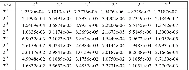
The absolute maximum errors in solution of Example 6 for0.5 and 0.5
h
\
2-6 2-7 2-8 2-9 2-10 2-11
2-1 2-2 2-3 2-4 2-5 2-6 2-7 2-8 2-9
1.2330e-04 3.1013e-05 7.7776e-06 1.9476e-06 4.8728e-07 1.2187e-07 2.1998e-04 5.5491e-05 1.3931e-05 3.4902e-06 8.7349e-07 2.1849e-07 1.5469e-04 3.6874e-05 8.9931e-06 2.2200e-06 5.5145e-07 1.3742e-07 1.0835e-03 3.1174e-04 8.3693e-05 2.1673e-05 5.5149e-06 1.3909e-06 6.9032e-03 2.1023e-03 5.8626e-04 1.5449e-04 3.9672e-05 1.0052e-05 2.6139e-02 9.0231e-03 2.6983e-03 7.4144e-04 1.9487e-04 4.9931e-05 5.6117e-02 2.9841e-02 1.0159e-02 3.0187e-03 8.2688e-04 2.1666e-04 4.9948e-02 6.1889e-02 3.1756e-02 1.0750e-02 3.1855e-03 8.7139e-04 1.6832e-02 5.5652e-02 6.4857e-02 3.2731e-02 1.1051e-02 3.2707e-03
VI. DISCUSSIONS AND CONCLUSIONS
We have described a special finite difference method for solving a singularly perturbed differential difference equation with layer behaviour at one end point. In the special second order method, we have used a second order finite difference approximation for second order derivative, a modified second order upwind finite difference approximation for first order derivative and a second order average difference approximation for y. This method controls the rapid changes that occur in the boundary layer region and it gives good results. To discuss the applicability of the method we have solved some model examples by taking different values of,and. We have presented maximum absolute errors for the standard examples chosen from the literature. The numerical solution is compared with the exact solution. It is observed from results that the present technique approximates the exact solution very well.
REFERENCES
[1] Prasad, H. S., Reddy, Y. N. (2012). Numerical Solution of Singularly Perturbed Differential- Difference Equations with Small Shifts of Mixed Type by Differential Quadrature Method, American Journal of Computational and Applied Mathematics 2012, Vol. 2, No.1, pp. 4652.
[2] Kadalbajoo, M. K., Sharma, K. K. (2004). Numerical analysis of singularly perturbed delay differential equations with layer behavior, Applied Mathematics and Computation Vol. 157, pp. 11-28. [3] Kadalbajoo, M. K., Sharma, K. K. (2008). A numerical method
based on finite difference for boundary value problems for singularly perturbed delay differential equations, Applied Mathematics and Computation Vol. 197, pp. 692-707.
[4] Kadalbajoo, M. K., Ramesh, V.P. (2007). Hybrid method for numerical solution of singularly perturbed delay differential equations, Applied Mathematics and Computation Vol. 187, pp. 797- 814.
[image:9.612.120.497.162.306.2] [image:9.612.120.495.343.483.2]International Journal of Emerging Technology and Advanced Engineering
Website: www.ijetae.com (ISSN 2250-2459, ISO 9001:2008 Certified Journal, Volume 7, Issue 9, September 2017)
390 [6] Kadalbajoo, M. K., Kumar, D. (2010). A computational method for
singularly perturbed nonlinear differential-difference equations with small shift, Applied Mathematical Modeling Vol. 34, pp. 2584-2596. [7] Bellen, A., Zennaro, M. (2003). Numerical Methods for Delay
Differential Equations, Oxford University Press, Oxford. [8] Driver, R. D. (1977). Ordinary and Delay Differential Equations,
Springer-Verlag, New York.
[9] Bellman, R. E., Cooke, K. L. (1963). Differential-Difference Equations, Academy Press, New York.
[10] El’sgol’ts, L. E. (1964). Qualitative Methods in Mathematical Analyses, Translations of Mathematical Monographs 12, American mathematical society, Providence, RI.
[11] Lange, C.G., Miura, R.M. (1985). Singular perturbation analysis of boundary value problems for differential difference equations, SIAM Journal of Appl. Math., Vol.45, pp. 687-707.
[12] Lange, C. G., Miura, R. M. (1994). Singular perturbation analysis of boundary value problems for differential difference equations, V. Small shifts with layer behavior, SIAM J. Appl. Math., Vol. 54, pp. 249-272.
[13] Duressa Gemechis File, Reddy Y. N. (2015). Domain decomposition method for Singularly perturbed differential difference equations with layer behavior.Int J EngApplSci,7(1),86-102.
[14] Sirisha, L., Phaneendra, K., & Reddy, Y. N. (2016). Mixed finite difference method for singularly perturbed differential difference equations with mixed shifts via domain decomposition. Ain Shams Engineering Journal.
[15] El’sgol’ts L. E., and Norkin, S. B. (1973). Introduction to the Theory and Applications of Differential Equations with Deviating Arguments, Academic Press, New York.
[16] M. Van Veldhuizen. (1979). Higher order schemes of positive type for singular perturbation problems, in P. W. Hemker, J.J.H. Miller, Numerical analysis of singular perturbation problems, Academic Press, New York, 361-383.
[17] O’Malley, R. E. (1974). Introduction to Singular Perturbations, Academic Press, New York.
[18] Lange, C.G., Miura, R.M. (1994). Singular Perturbation Analysis of Boundary Value Problems for differential difference equations, (VI), Small shifts with Rapid Oscillations, SIAM J. Appl. Math. , Vol. 54, pp. 273-283.