EMS Systems: Optimised Sensor Configurations for Control and Sensor Fault Tolerance

Michail, Konstantinos, Zolotas, Argyrios and Goodall, Roger M.

EMS Systems: Optimised Sensor Configurations for Control and Sensor Fault Tolerance

Original Citation

Michail, Konstantinos, Zolotas, Argyrios and Goodall, Roger M. (2009) EMS Systems: Optimised 

Sensor Configurations for Control and Sensor Fault Tolerance. In: In (STECH'09), International 

Symposium on Speed­Up, Safety and Service Technology for Railway and Maglev Systems 2009, 

16th ­ 19th June 2009, Niigata, Japan. 

This version is available at http://eprints.hud.ac.uk/id/eprint/17919/

The University Repository is a digital collection of the research output of the

University, available on Open Access. Copyright and Moral Rights for the items

on this site are retained by the individual author and/or other copyright owners.

Users may access full items free of charge; copies of full text items generally

can be reproduced, displayed or performed and given to third parties in any

format or medium for personal research or study, educational or not­for­profit

purposes without prior permission or charge, provided:

•

The authors, title and full bibliographic details is credited in any copy;

•

A hyperlink and/or URL is included for the original metadata page; and

•

The content is not changed in any way.

For more information, including our policy and submission procedure, please

contact the Repository Team at: [email protected].

*1 Department of Electronic and Electrical Engineering,

Loughborough University, Loughborough, Leicestershire, UK, LE11 3TU Email:{k.michail, a.c.zolotas, r.m.goodall}@lboro.ac.uk

The paper describes a sensor optimisation systematic framework approach and a Fault Tolerant control scheme for sensor failures applied to an EMS maglev system. The aim is to find the minimum number of sensors that can be used in order to optimise the performance, reduce complexity and offer sensor fault tolerance. The concept is verified via simulations with the non-linear model of an EMS system.

!

MAGLEV trains offer a number of advantages against the conventional wheel-on-rail trains [1]. A MAGLEV vehicle in contrast with the wheel-on-rails is suspended below the rail using electromagnetic forces. A number of types of MAGLEV suspension exist but in this paper the electromagnetic suspension (EMS) is considered. The EMS system uses attractive forces to support the vehicle and the passengers. This is a non-linear, unstable system with non-trivial requirements as well as a fail safe critical system and sensitive to sensor faults. In fact, if one or more sensors failures, most probably the EMS system instability and it will either fall off or stick to the track causing possible failures of the whole system. Being a critical fail-safe system substantially increases costs as it requires a " ault

olerant

ontrol (FTC) structure [2]. Previous work on optimised sensor configurations via

#

inear $ uadratic % aussian (LQG) control [3] is extended

to the FTC concept for sensor failures. Other approaches also exist from the sensor optimisation point of view including robust control [4] and robust stability via Loop shaping design procedure [5]. The optimised sensor configuration frameworks developed are based on the linearised model of the maglev suspension while simulations employ the actual nonlinear model for sensor selection performance validation.

f

H

Previous studies on FTC for MAGLEV suspensions have concentrated on state feedback control [6], LMI-based approaches [7], an encounter on simultaneous stabilisation [8], as well as duplex controllers to offer some form of hardware redundancy [9]. None of the previous studies has considered the sensor selection for optimum performance and fault tolerance. This paper presents a FTC approach which aims to reducing hardware sensor redundancy, while optimising the

overall MAGLEV performance (both in deterministic and ride quality terms).

f

H

The paper is organised as follows: Section 2 presents the non-linearities of the EMS system along with the state space linearization of the quarter car model. Section 3 presents the input disturbances to the MAGLEV suspension while the assigned objectives are given along with the required restrictions. In section 4 the sensor optimisation systematic framework via LQG is described and the extended sensor selection for fault tolerant control is given in section 5. Finally conclusions are drawn in section 6.

&

' ( ( ) * ( ) ) ( #

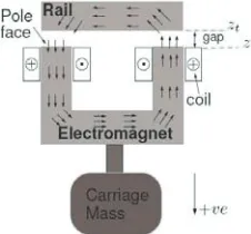
The diagram of an electromagnet suspension system is shown in Fig.1. The system represents a one degree of freedom model considered as a ‘quarter car’ vehicle equivalent. The suspension consists of an electromagnet with a ferromagnetic core and a coil which is attracted to the rail that is made out of ferromagnetic material. The carriage mass is attached to the electromagnet. is the rail position and

t

z

[image:2.595.364.477.524.629.2]

z is the carriage position. The air gap (z_tz), that is to be controlled to provide an appropriate suspension performance (see later).

Fig. 1 Diagram of 1DOF EMS suspension Assuming that the positive direction is downwards the equation of motion arising from Newton’s second law is

F Mg dt

z d

M ₂

2

carriage at the operating position. The electrical circuit of the electromagnet is given by

dt dB NA dt dI L RI

V_coil (2)

Where is the input voltage, is the coil’s resistance,

u R

Lis the leakage inductance, the number of turns and

N

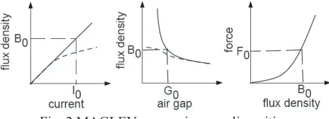
A is the pole face area. I is the coil current and is the flux density. As indicated in [10] the four important variables in the electromagnetic suspension are Force

B

F , flux density , the air gap and the coil current

B )

( : G0 z z

G t I . The

relationships between those variables are shown in Fig. 2 (straight lines for theoretical and dotted lines for a practical magnet including leakage and saturation). At constant air gap, the flux density is proportional to the coil current and at constant current is inversely proportional to the air gap.

[image:3.595.57.289.341.425.2]

Fig. 2 MAGLEV suspension non-linearities The force is proportional to the square of the flux density. The MAGLEV suspension is non-linear but there are no hard non-linearities in the system thus linear controllers can be used for control which can perform satisfactory as it is shown later in section 4.

To derive the LTI state space model, linearisation is performed around the operating point (nominal values) of the coil current , flux , force , nominal input voltage and air gap G

0

I B0 F0

0

V 0. The linearisation which leads

to the state space model in equation (3) can be found in [3]. x C y z B u B x A x m t dz u

g t

(3)

Note that subscript implies . The states are given as: where i is the coil current,

t

dz z_t

] ) ( [i z z z

x _t z is

the vertical velocity and (ztz) is the air gap. The state space matrices are given by (4), (5) and (6), where the measurements in the output matrix are the current, flux density air gap, velocity, acceleration . Different sensor combinations can be selected via defined as sensor sets. All feasible sensor sets are given by N

m

C )

(b (z)

m C

c=2Ns-1. Nc being the total number of sensors

sets and Ns is the total number of sensors (i.e for 5

sensors Nc=31 sensor sets).

The parameter values for the quarter car linear and non-linear model used are: M 1000kg

m

G0 0.015 B0 1T I0 10A F0 9810N

: 10

R L 0.1H N 2000 A 0.01m2.

» » » » » » » ¼ º « « « « « « « ¬ ª 0 1 0 0 0 ) ( ) ( M K K M K K NA K L NA K NA K L R

A b i b z z

i z z i g t t (4) » » » » » » ¼ º « « « « « « ¬ ª » » » » » ¼ º « « « « « ¬ ª 1 0 0 0

1 ( )

i z z dz i u NAK L NA K B NA K L B t t (5) » » » » » » » ¼ º « « « « « « « ¬ ª M K K M K K K K C z z b i b z z i m t t ) ( ) ( 0 0 1 0 1 0 0 0 0 0 1 (6) + ! ( , ! ' ( ) % # ( ! , ( ( $ ! ( ) ( +

./ 0 1 2 3 .40 45 6 7 .3

The stochastic inputs are due to random variations of the rail position as the vehicle moves along the track. These arise due to track-laying inaccuracies, steel rail discrepancies as well as due to unevenness during the installation of the rails. Considering the vertical direction, the velocity variations can be approximated by a double-sided power spectrum density (PSD) expressed as:

vechcle r dz AV S

t S (7)

Where is the vehicle speed (taken as 15m/s in this case) and represents the roughness and is assigned a value of for high quality track. The corresponding autocorrelation function is then given as:

vehicle V r A 7 10 1u ) ( 2 )

(W S2ArVvehicleG W

R (8)

+

& 8 .8 9 : 45 43 .40

5 6 7 .

The main deterministic input to the suspension in the vertical direction is due to the transition onto a gradient. In this work, the deterministic input shown in Fig. 3 is used that represents a gradient of at a vehicle speed of , an acceleration of and a jerk of .

% 5 s

m/

15 0.5m/s2

3

[image:4.595.320.519.102.250.2]

/ 1m s

Fig. 3. Deterministic input to the suspension with 15m/s onto 5% track gradient

+ +

8 3 4; 5 8 < 7 49 8 : 8 5 .3

Fundamentally there is a trade off between the deterministic (track gradient) and the stochastic response (ride quality) of the suspension. For slow speed vehicles, performance requirements are described in [11, 12]. The objective is to minimise both the vertical acceleration, (improve ride quality) and the excitation of the electromagnets by minimizing RMS of the current variations about the nominal point. Therefore, the conflicting objective functions are formally written as:

rms z

) (i_rms

rms

rms z

i 2

1 , I

I (9)

The working limitations for the MAGLEV suspension are listed in Table 1. The assigned constraints guarantee that the MAGLEV suspension is working within safety limits.

In any real application the sensors add noise to the measured quantities. For the MAGLEV suspension, the noise from sensors can be amplified by the controller and appears on the control signal (at the driving signal of the suspension). Particularly, if the controller has high gains, then the amplitude of the noise can become very large. Figure 4 shows the open-loop frequency response from the control input to the air gap and the current . It can be seen that the open-loop frequency response has a low pass filter characteristics and therefore the noise is filtered having limited effect at the outputs. Although the MAGLEV suspension can be considered as a low pass filter, it is better to keep the level of the noise as low as possible with an extra constraint added to the optimisation algorithm:

)

(u (z_tz) )

(i

V u_noise50 .

[image:4.595.78.262.203.340.2]

Fig. 4 Frequency response from uto i/(ztz)

Table 1 MAGLEV suspension constraints Constraints Value RMS acceleration (zrms) < 0.5ms-2 RMS gap variation,((ztz)rms) < 5mm Control effort, (u_rms) < 300V(3IoRo)

Air gap deviation,((ztz)p) < 7.5mm Control effort, (up) < 300V(3IoRo)

Settling time, (ts) < 3s

Steady state error (e_ss) =0

= > ? @ A ? B C B D E FG F ? H E F B A I FH J K L

In this section, the optimised sensor configurations for the MAGLEV suspension are presented. The details of the systematic approach are discussed in [3]. The overall block diagram of the sensor optimisation via LQG is depicted in Fig. 5. Details for controlling non-linear models via linearised controllers but can be found in [13]. The overall problem is formulated into a multiobjective constraint optimisation with two objective functions in (9) minimised subject to the constraints listed in Table 1. The problem is solved for every possible sensor set and therefore a genetic algorithm [14] approach is employed [3].

The LQG controller tuning is performed according to the separation principle [15]. The first step is to tune the

J

inear

K

uadratic

C

egulator (LQR) and select the ‘ideal’ state feedback gains(Kr)which represents the desired or ‘ideal’ performance. The second part is where the sensor information becomes critical. The Kalman estimator is tuned to achieve the ‘ideal’ performance (LQR selected response) for every sensor set (i.e sensor optimisation).

Consider the following state space expression

K

Z

Z

x C y

B u B x A x

m

d dz u

g t

[image:4.595.305.538.303.422.2]

Where, Z_d and Z_Kare the process and measurement noises respectively. These are uncorrelated zero-mean Gaussian stochastic processes with constant power spectral densities W and respectively. In particular, the problem is to find which minimises the performance index (11) [15] for each sensor set (this particularly relates to the information provided to the Kalman filter).

V

[image:5.595.314.522.180.333.2]

y s K u LQG( )

Fig. 5. Sensor selection via LQG control

>

°¿ ° ¾ ½

°¯ ° ® ­

³

f o

T

T T T

LQG x Qx u Rudt T

E J

0

1

lim

@

(11)

Here, and are the state and control weighting functions with and of the linear quadratic part of the LQG. Similarly, W andV are the tuning parameters of the Kalman filter part. For appropriate disturbance rejection the LQR part is designed on an augmented system with the extra integral state of the gap (however the Kalman filter is designed on the original state space matrices, but the integral state is later provided by the selector matrixC ).

Q R

0 t T Q

Q T t0

R R

s

It is also worth noting that for the LQR design we choose output regulation, i.e. accelerationz, air gap(z_tz) and the integral of the air gap (the last quantity specifically refers to the speed of response). Thus, is in fact given by where is the output matrix selecting the above regulated signals, i.e.

³

(z_t z)

Q

z z T zQC C

Q C_z

>

z (z_t z)

_³

(z_tz)

@

and is the corresponding weight. The Kalman filter is designed such that

is minimised. z Q

¿ ¾ ½ ¯

®

­ š š

] [ ] [x x x x

E T

The Pareto optimum of controllers for the LQR tuning is depicted in Fig. 6. The trade off between the ride quality and the input excitation current is obvious, i.e to reduce

the acceleration for the stochastic response more input power is required. For the Pareto optimum front of controllers any one can be selected that suits the user’s need. For the concept presented in this paper, the state feedback gains that result in the best ride quality are selected with the following feedback gains:

1 5 5

1 3

/ 10 41 . 2 ,

/ 10 14 . 2

/ 10 36 . 3 ,

/ 8 . 246

), ( ),

(

, ,

u u

u

³

V mK V ms

K

ms V K

A V K

V z t z V

z t z

V z V

i

r r

r

r

[image:5.595.59.287.208.390.2]

(12)

Fig. 6. Pareto optimum front of controllers for LQR The resulting deterministic response of the MAGLEV suspension is illustrated in Fig. 7. The transition onto the track gradient clearly relates to the working boundaries listed in Table. 1, i.e. steady state error, maximum air gap deviation etc. Note that the input voltage to the maglev suspension is limited to around 80V which is within preset limits as indicated on Table 1.

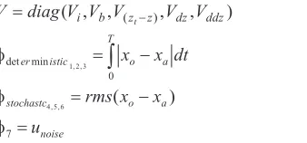
[image:5.595.360.485.435.558.2]

) , , , ,

(Vi Vb V(z z) Vdz Vddz diag

V _t (13)

³

I _{er istic} T x_o x_adt

0 min

det 1,2,3 (14)

) (

6 , 5 ,

4 o a

stochastc rms x x

I ₍₁₅₎

noise

u

I7 (16)

Note, that in (13) subscript and . is the vector of monitored states of interest of the closed loop with the LQR state feedback, and the vector of monitored states of interest of the closed loop with the overall LQG controller [e.g. actual closed loop (prior to adding sensor noise]. This makes a total of 6 individual objective functions.

z

dz ddz z x_o

a x

Evolution is followed in 5 generations with a population of 25 individuals. After the simulations, there are 775 optimum individuals from which to choose the best. The selection procedure of the optimally tuned Kalman estimator is based on the overall constraint violation function [3]. This function indicates if there is a constraint violation or not. After the Kalman tuning for a corresponding sensor set, there are 25 tuned Kalman filters to choose from. The best Kalman selection at this point is done according to the precision of the state estimation which is given as the sum of the objective functions

) (:

¦

6

1

min

det , )

( i

stochastic istic

er

S I I (17)

This procedure gives an optimum controller for each sensor set, with 24 out of 31 sensor sets found to meet all constraints. Table 2 illustrates the results for six sensor sets and the corresponding response of the optimally tuned LQR controller. The sensor combinations that satisfy all constraints are marked (¥). As it can be seen from Table 2 a variety of sensor sets can achieve the ‘ideal’ performance. The concept of the optimised sensor configurations scheme can be extended to the fault

tolerant control for sensor failure using the overall information from the final results given.

M > ? @ A ? B C ? @ J @ N E F B A O B C O E N

The information from sensor optimisation framework can be used in order to apply FTC for sensor failures with an attempt to minimise the sensor hardware redundancy with maximum performance for every possible sensor set under faulty conditions. Such concept is depicted in Fig. 9. Assuming that control is with Id:8, using the information extracted from Table 2, a bank of controllers can be used in order to restore performance following one or multiple sensor faults. In fact, the suspension performance, after reconfiguration after a sensor fault, is easily predicted from the data listed in Table 2. According to this table, for example, when four measurements fail and the air gap remains there is a serious air gap constraint violation (see Id:4). Although is not likely for four sensors to fail at the same time, this shows that a critical fail safe system might require, some form of hardware or analytical redundancy for the air gap signal.

[image:6.595.82.251.100.179.2]

The alternative approach is to avoid use of the air gap measurement. Particularly, assume that the worst case is to remain with one measurement (i.e Id:1, Id:2 and Id:3). According to the given data if a sensor remains after some sensor failures the performance is satisfactory. From this point of view, the Id:6 can be used instead of the full sensor set. Note that Id:6 and Id:8 have very similar performance. Therefore, if Id:6 is used, then the worst resulting performance when both b and z fail, is the response with Id:1 which has steady state violation but it can be safely used until the vehicle decelerates and is maintained. At this point, any method can be used for the reconfiguration mechanism. When Kalman estimators are used, a common approach for the fault detection is to use the residual. After a fault occurs, the fault is detected, isolated and the controller is reconfigured as illustrated in Fig. 9.

Table. 2 Sensor Optimisation results via LQG control

Sensor set (zt z)rms urms zrms (zt z)p up ts ess

Id Sensors mm V ms-2 mm V s mm

LQR response ĺ 1.5 21.83 0.31 7.3 52.4 2.16 0.019 ¥ 1 i 1.75 29.32 0.5 2.09 22.85 6.18 P

>Q R

x 2 b 1.42 22.51 0.31 6.74 63.82 2.18 0.019 ¥ 4 (ztz) 1.45 22.39 0.31

Q

P

>S T

84.83 2.56

Q >

P

T

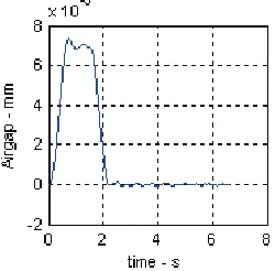
[image:6.595.61.538.569.713.2]

Fig. 9. FTC for EMS system with sensor failure/s The fault scenario is that the accelerometer is giving wrong readings starting at t=1sec. The FTC scheme detects the faulty measurement and reconfigures the controller in order to restore the performance using the remaining two sensors (i.e ). The performance is immediately recovered by reconfiguring the controller and the responses of healthy and faulty situations are illustrated in Fig. 8 (stability is implicit as we assume negligible switching time).

b i,

[image:7.595.78.271.399.540.2]

The input voltage is limited to the required working boundaries with the noise amplitude been limited to very low amplitude after the Kalman filtering properties.

Fig. 8. Air gap response prior to a sensor fault.

S > N B A N J U ? F B A ?

The concept presented in this paper shows that the sensor selection with respect to MAGLEV suspension optimum performance with sensor fault tolerance is important. The overall approach illustrate that three sensors can be used instead of the max five which results in: the minimum number of sensors used with optimum performance, a reduction of control system complexity, and offers sensor fault tolerance and optimum performance for every possible sensor set prior to fault conditions. The overall cost can be therefore reduced, although this is not considered here. However, the results show the efficacy of the framework which can be adapted to other applications and related performance specifications.

C @ O @ C @ A N @ ?

[1] Hyung-Woo, L. Ki-Chan, K. and Ju, L.: Review of maglev train technologies. IEEE Transactions on Magnetics, 42(7), 1917-1925 (2006)

[2] Blanke, M. Izadi-Zamanabadi, R. Bogh, S.A. Lunau, C.P.: Fault-tolerant control systems - a holistic view, Control Engineering Practice, 5(5), 693-702 (1997) [3] Michail, K. Zolotas A.C. and Goodall, R.M.: Optimised sensor configurations for a MAGLEV suspension, 17th IFAC World Congress, 8305-8310 (2008)

[4] Michail, K. Zolotas A.C. and Goodall, R.M.: Sensor optimisation via H’ applied to a MAGLEV suspension system. WASET: International Conference on Control, Automation and Systems. vol. 31, 171-177, (2008) [5] Michail, K. Zolotas A.C. and Goodall, R.M.: MAGLEV suspensions - a sensor optimisation framework, IEEE 16th Mediterranean Conference on Control and Automation. 1514-1519, (2008)

[6] Huixing, C. Zhiqiang, L. and Wensen, C.: Fault tolerant control research for high-speed maglev system with sensor failure, in 6thWorld Congress on Intelligent Control and Automation, vol. 1, 2281–2285, (2006). [7] Sung, H. K., Lee, S. H., and Bien, Z.:, Design and implementation of a fault tolerant controller for ems systems, Mechatronics,, 15(10), 1253–1272, (2005). [8] Zhang, Z., Long, Z., She, L., and Chang, W.: Fault - tolerant control for maglev suspension system based on simultaneous stabilization, IEEE International Conference on Automation and Logistics, 299–303, (2007)

[9] Kim, H-J. Kim, C.-K. and Kwon, S.: Design of a fault - tolerant levitation controller for magnetic levitation vehicle, International Conference on Electrical Machines and Systems, 1977–1980 (2007).

[10] Goodall, R.M.: Generalised design models for EMS MAGLEV, 20th International Conference on Magnetically Levitated Systems and Linear Drives, (2008) (Available at: http://www.maglev.com)

[11] Goodall, R.M.: Dynamic characteristics in the design of MAGLEV suspensions. Proceedings of the Institution of Mechanical Engineers, Part F: Journal of Rail and Rapid Transit, 208(1), 33-41, (1994)

[12] Goodall, R.M.: Dynamics and Control requirements for EMS MAGLEV suspensions. Proceedings on International Conference on MAGLEV, 926-935, (1994) [13] Frieland, B.: Advanced control system design, Prentice-Hall Inc, (2004)