Time resolved noise source analysis in subsonic turbulent jets

(1)

TIME-RESOLVED NOISE SOURCE ANALYSIS

IN SUBSONIC TURBULENT JETS

David E. S. Breakey

May 2014

Department of Mechanical and Manufacturing Engineering Parsons Building, Trinity College

Dublin 2, Ireland

(2)

(3)

Declaration

I declare that this thesis has not been submitted as an exercise for a degree at this or any other university, and it is entirely my own work.

I agree to deposit this thesis in the University’s open access institutional repository or allow the library to do so on my behalf, subject to Irish Copyright Legislation and Trinity College Library conditions of use and acknowledgement.

(4)

(5)

At the tumultuous noise peoples flee; when you lift yourself up, nations are scattered, – Isaiah 33:3

(6)

(7)

Abstract

For over sixty years, researchers have been trying to understand and predict jet noise emissions, seeking to reduce perceived noise levels for passengers and those who live and work near airports. The complexity of jet noise source mechanics has meant that an adequate theory of jet noise—one yielding predictions sufficiently accurate to fully incorporate noise concerns into the aircraft design cycle—does not yet exist.

This thesis contributes to the understanding of jet noise sources by developing and testing tools for the time-resolved analysis of jet noise sources. The time-resolved approach provides extra insight that is masked in a purely statistical analysis of the source dynamics.

First, time-resolved Particle Image Velocimetry is used to directly correlate jet velocity fluctuations with out-of-flow sound signals, yielding two principal advantages over traditional velocimetry techniques: temporal resolution of the development of individual flow features; and an estimate of the space–frequency coherence. The measured time-domain quantities are accurate, but in the frequency domain, errors arising from a combination of high-frequency aliasing and signal noise make the estimates inaccurate. Nonetheless, the correlation signature in a low-speed jet with a Mach number of 0.25 is shown to be consistent with a large-scale oscillatory source called a wavepacket.

(8)

on the Green’s function solution of wavepacket fluctuations is used with the near-field data to obtain far-field predictions, but the agreement with measurements is not good for the jet studied. This is shown to be the result of the appearance of a spurious source artificially introduced by the finite extent of the microphone array used in the measurements, an effect expected to be smaller for higher-Mach-number jets. Despite this shortcoming, the existing technique is extended to provide time-domain far-field pressure predictions. The technique is demonstrated using an artificial dataset, but it will be necessary to treat the problem of the spurious source before meaningful results for experimental data can be obtained.

Third, a structural similarity metric originating from image compression analysis is adapted for time-resolved aeroacoustic signals. When faced with common types of aeroacoustic errors, the new metric outperforms traditional quantitative metrics for comparing the similarity between signals, providing better discrimination between error types while remaining resilient to contamination by random signal noise. Such a metric shows promise for optimization-based development of noise source prediction schemes.

(9)

Acknowledgements

This project was conceived by Prof. John Fitzpatrick, who also guided me in its early stages. I am indebted to John for his insight and experience in navigating the problem of jet noise and the maze of academia. It is only unfortunate that he did not live to see me through to the end. I also thank Dr. Craig Meskell for taking me on as his student after John’s death. Craig’s careful guidance, creative insight, and patient oversight during the analysis of the data and dissemination of the results, particularly the compilation of this thesis, have benefited me greatly.

From my colleagues in Trinity, I would particularly like to thank Drs. John Mahon, Rayhaan Farrelly, and Shane Finnegan for teaching me experimental techniques. I also thank Miguel Garcia-Pedroche for his help in obtaining the TR-PIV data.

For the work on wavepackets, foremost I thank Drs. Peter Jordan and André Cavalieri, who introduced me to wavepacket analysis. Particularly, I thank Peter for hosting me in theCentre d’études aérodynamiques et thermiques(CEAT) in Poitiers, France so that I could perform my experimental campaign. Peter and André also helped in the collection of the pressure data and—perhaps most importantly—included me in their discussions of the mystery of wavepackets and the jet noise puzzle. They also guided me in the analysis of the current data and the development of my wavepacket analysis techniques. I would like to thank Dr. Olivier Léon for providing the code for the statistical predictions of the far-field emissions of near-field wavepackets. I also thank Dr. Daniel Rodríguez and Prof. Tim Colonius for their provision of the Parabolised Stability Equation solutions of the analyzed jet flow.

(10)

(11)

Prior publications

Many of the ideas and figures contained in this thesis have been previously presented in the following publications:

Breakey D& Meskell C (2013)Comparison of metrics for the evaluation of similarity in acoustic pressure signals.Journal of Sound and Vibration332(15):3605–3609.

Breakey DES & Fitzpatrick JA (2012) Time-resolved PIV for aeroacoustic source analysis. In: 16th International Symposium on the Application of Laser Techniques to Fluid Mechanics, Lisbon, Portugal.

Breakey DES, Fitzpatrick JA, & Meskell C (2013a)Aeroacoustic source analysis using time-resolved PIV in a free jet.Experiments in Fluids54(5):1–16.

Breakey DES, Jordan P, Cavalieri AVG, Léon O, Zhang M, Lehnasch G, Colonius T, & Rodríguez D (2013b)Near-field wavepackets and the far-field sound of a subsonic jet. In: 19th AIAA/CEAS Aeroacoustics Conference, Berlin, Germany.

(12)

(13)

List of figures

Chapter 2 2.1 Turbulent jet schematic . . . 10

(17)

LIST OF FIGURES

2.3 Sound propagation through a mean jet flow profile. . . 17

2.4 Theorized noise components of a jet . . . 20

Chapter 3 3.1 Hot-wire anemometry probes . . . 29

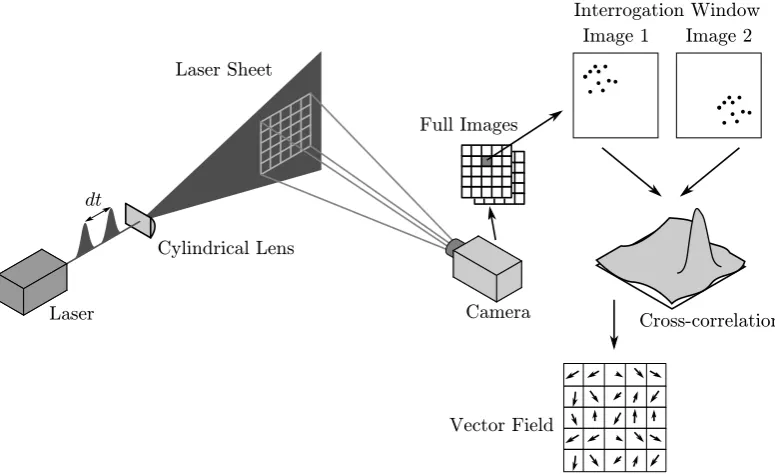
3.2 Schematic of the Particle Image Velocimetry technique . . . 31

3.4 Example usignal histogram . . . 42

3.5 Wavelet filtering of microphone signals in jet near-field . . . 46

3.6 Comparison between space–time resolution of TR-PIV and HWA-basedu0p0 correlation quantities . . . 48

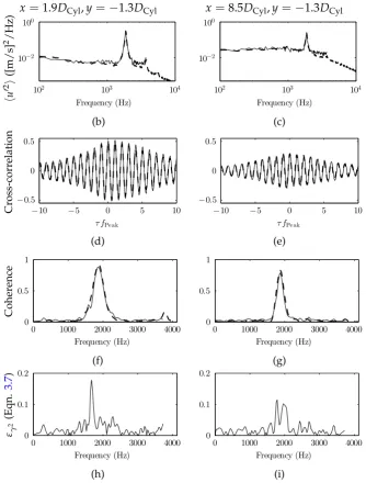
3.7 Free jet axial velocity spectra . . . 49

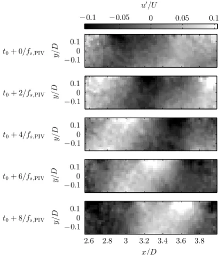
3.8 Example TR-PIV time series ofu0 for the free jet flow . . . 50

3.9 Cross-correlation coefficient between u0 (q0 for simulation) and the acoustic part of p0 . . . 51

3.10 Source model for correlation simulation . . . 51

Chapter 4 4.1 Schematic representation of a snapshot of a wavepacket and its sound radiation in a jet . . . 58

4.2 Schematic representation of wavepackets at different convection velocities and their corresponding k–f spectra . . . 63

4.3 Comparison between linear PSE predictions and measuredu0 for the axisymmetric mode on the jet centreline . . . 65

4.4 Comparison between linear PSE predictions and measured u0 at three axial stations . . . 66

4.5 Overview of 4-ring setup . . . 67

4.6 7-ring near-field azimuthal array setup (7pt correlation) . . . 68

4.7 4-ring near-field azimuthal array setup (2pt correlation) . . . 69

4.8 Energy distribution and cumulative sum for the first 10 POD modes ofPm,ω for m

=

0 from the 4-ring array measurements . 71 4.9 Comparison of PSE estimates and measured autospectra magni-tudes ofPm,ω for m

=

0 and M

=

0.6 . . . 72

(18)

4.11 m

=

0 POD modes ofPm,ω for 4-ring and 7-ring setups . . . 75

4.12 Comparison between near-field and far-field m

=

0 pressure mode signals ( ˜pm) for both full signal and POD reconstruction . 76

4.13 Normalized retarded correlation between near-field ˜p0 and

far-field ˜p0. . . 77

4.14 Individualm

=

0 POD mode contributions to near-field–far-field correlation for 7-ring data. . . 78

4.15 Cumulative m

=

0 POD mode near-field–far-field correlations for 7-ring data . . . 78

4.16 Individualm

=

0 POD mode contributions to near-field–far-field correlation for the reduced-order projection . . . 79

4.17 Cumulativem

=

0 POD mode near-field–far-field correlation for the reduced-order projection . . . 79

4.18 Geometric considerations for time-domain predictions with a finite-window Fourier transform. . . 81

4.19 Effect of experimental near-field array truncation on the statistical far-field Green’s function prediction . . . 82

4.20 Effect of experimental near-field array truncation on the time-domain far-field Green’s function prediction. . . 83

4.21 Snapshot comparison between Lighthill integral solution and Green’s function prediction for wavepacket sound emissions with a truncated near-field array. . . 85

4.22 Comparison of Green’s-function-predicted directivities from the current 4-ring measurements . . . 87

Chapter 5

5.1 Process model for current study . . . 96

5.2 Sample comparison between p

(

t

)

and ˆp

(

t

)

for the different error types . . . 97

5.3 Results from metric tests with simulated data . . . 102

5.4 Results from metric tests with experimental far-field data . . . . 102

Appendix A

(19)

LIST OF TABLES

A.2 Ratio of axial (u0) to radial (v0) turbulence intensity along free jet centre-line . . . 114

Appendix B

B.1 Analysis procedure for time-domain far-field signal prediction . 117

B.2 Validation results for the far-field Green’s function predictions from the near-field array . . . 118

B.3 Effect of M and rA on the far-field statistical predictions with

different CSM models . . . 120

List of tables

Chapter 3

3.1 Summary of experimental parameters . . . 40

3.2 Summary of source simulation parameters . . . 52

Chapter 4

4.1 Experiment conditions for both experimental campaigns . . . . 67

Chapter 5

5.1 Error expressions for metric comparison . . . 99

5.2 Metrics used in similarity analysis . . . 99

Appendix B

B.1 Model constants used in validation problem . . . 116

(20)

(21)

Nomenclature

Functions and variables

γ2_ab(ω) Coherence function

δ(·) Dirac delta function

δij Kronecker delta function,δij =1 when i= jandδij =0 wheni6= j

θ Observer angle measured from downstream jet axis

λ Wavelength

µ Dynamic fluid viscosity

ρ Fluid density, mass per unit volume

σa Root-mean-square of a data series,i.e.σa =RMS[a(t)]

τ Time lag

τr Retarded time lag,τ− |xo−xs|/c0 Ψ(ζ) Wavelet mother function

ω Angular frequency, 2πf

a,b Generic time-series variables,i.e. a(t),b(t)

c0 Speed of sound in ambient reference conditions

D Jet diameter

dB Decibels

f Frequency

Gaa(f) Autospectral density ofa

Gab(f) Cross-spectral density betweenaandb

k Wavenumber, 2π/λ

M Mach number,U/c0

(22)

Raa(τ) Autocorrelation function of awith time lagτ

R_ab(τ) Cross-correlation function between aandbwith time lagτ

Re Reynolds number,ρJUD/µJ

s Wavelet scale

t Time

Tij Lighthill stress tensor

U Mean jet velocity at the centre of the nozzle exit

u,v,w Velocity component in x,y,zdirection, respectively

Wi,PIV PIV interrogation window length in theidirection

x,r,φ Spatial coordinates in a cylindrical reference frame anchored at the

centre of the jet exit

x,y,z Spatial coordinates in a Cartesian reference frame anchored at the centre of the jet exit

xo Observer location

xs Source location

Operators

∗ _{Complex conjugation}

Designates time-averaged part of quantity,i.e. a=a+a0

0 _{Designates time-fluctuating part of quantity,}_{i.e. a}₌_a₊_a0

h i Ensemble average

Subscripts

0 Value taken at ambient reference conditions

c Value for convection quantity

i,j,k Vector indices

J Quantity measured at jet exit

o Denotes observer location

RMS Root-Mean-Square

(23)

NOMENCLATURE

Acronyms

ACARE Advisory Council for Aviation Research and Innovation in Europe

AOI Area Of Interest

BBSAN Broadband Shock Associated Noise

CFD Computational Fluid Dynamics

CSM Cross-Spectral Matrix

CTA Constant Temperature Anemometry

CWT Continuous Wavelet Transform

DNS Direct Numerical Simulation

DWT Discrete Wavelet Transform

EPNdB Effective Perceived Noise Decibels

EPNL Effective Perceived Noise Level

FOV Field Of View

FSS Fine-Scale Similarity

HWA Hot-Wire Anemometry

ICAO International Civil Aviation Organization

LDA Laser Doppler Anemometry

LES Large Eddy Simulation

LSS Large-Scale Similarity

LST Linear Stability Theory

MSE Mean-Square-Error metric

MSSIM Mean SSIM

PIV Particle Image Velocimetry

PNL Perceived Noise Level

PNLT Tone-corrected Perceived Noise Level

POD Proper Orthogonal Decomposition

PSE Parabolized Stability Equations

RANS Reynolds-averaged Navier–Stokes

(24)

RMS Root-Mean-Square

SPL Sound Pressure Level

SSIM Structural Similarity Metric

TR-PIV Time-Resolved PIV

WSSIM Time–frequency Weighted SSIM

(25)

Chapter 1

Introduction

1.1 Context for jet noise research

Today, the aviation industry is at the heart of culture and commerce worldwide, con-necting communities and businesses to an extent that could not have been conceived of only a century ago. The International Civil Aviation Organization (ICAO) notes that airlines carried 2.3 billion passengers and 38 million tonnes of freight in 2009, and air traffic is expected to grow steadily for the foreseeable future (ICAO-ER,2010). Such growth generates significant challenges as the aviation industry seeks to adapt to global needs for more sustainable and accessible air transport. One of the most im-portant of these challenges is reducing the noise emitted by aircraft, particularly near airports, where the most significant community opposition to airport expansion and operation arises from noise concerns (ICAO-ER,2010). In response to this challenge, the Advisory Council for Aviation Research and Innovation in Europe (ACARE) has set an ambitious goal for noise reductions by 2050: a 65% reduction in perceived noise levels relative to the year 2000 (ACARE-SRIA,2012). Similar goals have also been put in place by similar agencies worldwide.

(26)

engine with the ambient air (Viswanathan, 2010). This noise component, calledjet noise, is generated by aerodynamic phenomena rather than mechanical phenomena such as engine vibrations.

The study of the aerodynamic generation of sound—or aeroacoustics—began with the foundational work of Lighthill (1952) over sixty years ago. In part due toLighthill’s (1952) work, aircraft today are significantly quieter than those manu-factured at that time; however, aircraft noise concerns are just as important as ever, and the source mechanisms of jet noise are not well enough understood to fully in-corporate noise concerns into the aircraft design cycle. Noise predictions are possible but difficult to verify before the testing and prototyping stages, and they are highly reliant on empirical constants. Accurate numerical simulations are possible for simple jets, but their computational expense is too great for use as prediction tools, and they do not contribute directly to the understanding of jet noise source mechanisms since they can determine if a jet is louder or quieter but not specifically why. Fledgling noise reduction technologies take decades to incorporate into production aircraft and the noise reductions have been moderate. An adequate theory of jet noise requires the understanding of noise source mechanisms in jets necessary to create accurate, robust noise source models and the predictive power necessary to incorporate noise concerns directly into the aircraft design cycle. Such a theory will pave the way toward significant practical jet noise reductions.

1.2 Project context and overview

1.2.1 Toward time-resolved jet noise source analysis

(27)

1.2. PROJECT CONTEXT AND OVERVIEW

Though tracking or describing turbulence in real time is not a feasible proposition, like many real-life engineering challenges, practical jet noise reduction may not necessarily result simply from adding more information to jet noise models, but from carefully interpreting the information that is already available using current measurement techniques. This extra understanding available from a time-domain perspective may lead to novel noise reduction devices and strategies that would not have been developed looking only at a statistical picture of a jet’s noise emissions.

1.2.2 Objectives

This thesis develops techniques for time-resolved analysis of jet noise sources and far-field sound. The objectives of this project are to

• determine the utility of a space-resolved and time-resolved Particle Image Ve-locimetry to a low-speed jet and use it to interpret in-flow sound source signa-tures,

• detect the signatures of large-scale structures in the near-field of a subsonic jet and use the near-field signatures to predict the far-field sound in the time domain,

• and develop a comparison tool for evaluating the similarity between time-domain aeroacoustic signals.

These objectives have been met and the results of each are presented in chapters3,4, and5, respectively.

1.2.3 Progress beyond the state of the art

(28)

Finally, chapter 5 is the first application of a comparison metric for time-domain aeroacoustic signals that is suitable for use in quantitative comparison of time-domain aeroacoustics signals, which could be used to help isolate acoustically important noise model parameters.

Though this work does not claim to solve the problem of jet noise, following in the footsteps of a long series of gifted researchers, it constitutes another step on the path to a truly adequate theory of jet noise, which will contribute to the achievement of the long-term noise reduction goals of the aviation industry.

1.3 Thesis overview

(29)

Chapter 2

Background

2.1 Aims of jet noise research

Jet noise emissions are an important aspect of aircraft design, but they are not the only challenge facing aircraft designers. The design process in aeronautics is fraught with compromises, and improvements in one aspect of an aircraft’s design frequently have negative impacts on other design concerns. The primary aim of jet noise research is to achieve jet noise reductions with minimum negative impact on other factors of the aircraft design. These factors include aircraft weight, performance (i.e. thrust), fuel consumption, and cost. The design modifications necessary to achieve these reductions must not adversely affect the other design concerns beyond an acceptable level. However, the current tools available to jet noise researchers do not allow an accurate prediction of the jet noise emissions of a novel engine design at the concept stage, requiring lengthy iterative testing of new designs, hindering the designer’s ability to incorporate jet noise concerns into the design cycle. Therefore, a more complete theory of jet noise is required that has the following characteristics:

Understanding The sources of noise in turbulence should be identified so as to under-stand what makes a turbulent flow efficient at generating and radiating sound. The propagation of noise through a turbulent flow should also be understood so that the known sound source field can be interpreted as meaningful far-field noise emissions.

(30)

Despite approximately sixty years of jet noise research since Lighthill’s (1952) seminal paper, neither of these capacities is close to being adequately fulfilled. Practical jet noise reduction is still largely experimental and iterative, which is expensive and inefficient. As researchers continue to pursue an adequate theory, jet noise promises to be an active field of aeronautical research for many years to come.

Though these criteria have not yet been fulfilled, much progress has been achieved by the jet noise community in the last sixty years. The basic features of jet noise have been identified, as well as many qualitative and quantitative effects. For example, Lighthill’s (1952) original paper led to approximate scaling laws showing the sound emissions increase exponentially with jet speed, and new larger-diameter, lower-speed engines have made jets significantly quieter than comparable aircraft from the 1950s and 1960s (see§ 2.2.4). Simplified models of the sound sources in jets have also helped identify the importance of various jet design parameters. Also significant is the fact that, through decades of work, a considerable experimental database now exists in the literature evaluating jet designs at many different operational parameters, providing the opportunity for current and future researchers to make robust comparisons across a broad spectrum of jet types.

Finally, it is important to note that practical noise reductions do not require a complete time-resolved description of the far-field sound accurate to the measurement error of sound measurement equipment—such as could be achieved by direct solution of the equations of fluid motion—rather, it is only necessary that aircraft designers have the information necessary to compare jet designs based on their ability to meet regulatory noise limits and that the designers have enough confidence in this information to make informed design decisions. Hybrid solutions that begin by calculating the mean hydrodynamic field, which can be calculated in a reasonable time (e.g. Reynolds-Averaged Navier–Stokes (RANS) simulations), and then apply appropriate source models would be nearly as useful—and more practically feasible— to jet designers as complete solutions that require much higher computational cost.

2.2 Introduction to acoustics and aeroacoustics

2.2.1 What is sound?

(31)

2.2. INTRODUCTION TO ACOUSTICS AND AEROACOUSTICS

stagnant fluid—also called a quiescent fluid—is given as1 (e.g. Hirschberg,2001)

1 c2 0

∂2p0 ∂t2 −

∂2p0 ∂x2_i

=0, (2.1)

wherec0 is the speed of sound in the fluid reference state, pis the local fluid pressure, tis time, xi is the x-coordinate in theidirection. The0 denotes the fluctuating part of the variable2. Equation (2.1) applies only when there are no sources of sound in the medium since there is no source term on the right hand side. The importance of the wave equation is that it shows that all sound propagates atc0. In contrast to sound,pseudo-sound(Rienstra & Hirschberg,2010) is a pressure fluctuation that does not satisfy the wave equation (i.e. does not propagate at c0). Pressure fluctuations due to sound in an otherwise quiescent fluid can therefore all be classified as sound, while fluctuations in a non-quiescent fluid, such as in turbulent regions in a jet, can be made up of both sound and pseudo-sound components. The part of a fluid’s motion that is sound is often called the acoustic component, while the pseudo-sound part is the hydrodynamic component. Separating the two components in jet flows is usually non-trivial.

While acoustics is the study of sound in general, aeroacoustics is the study of sound generated by flow phenomena. Whereas acoustic sources arise from external phenomena, aeroacoustic sources are governed by the same fluid dynamical equations as the sound propagation itself. Since aeroacoustic sources are governed by these same equations, the principal difficulty in aeroacoustics is separating the fluctuations constituting an aeroacoustic source from other fluctuations in the flow that do not cause acoustic emissions.

Though the Navier–Stokes equations—which are thought to fully describe both hydrodynamic and acoustic fluid motion—are well known, the complexity of solving the acoustic solution for problems of practical interest is too great. This is complicated by the fact that the acoustic energy emitted by aeroacoustic sources is generally several orders of magnitude lower than that of the hydrodynamic fluctuations, meaning that the precision required in the analysis of aeroacoustic problems is several orders of magnitude finer than comparable aerodynamic problems. This is additionally compli-cated by the fact that high-frequency flow information, which is of little importance in aerodynamics, is especially important in aeroacoustics.

Though direct solutions of the Navier–Stokes equations can be obtained by

Com-1_{Equation (2.1)} _{can be generalized for a fluid undergoing arbitrary motion as is described by}

Hirschberg(2001) and in§ 2.2.4. It follows that, for a non-quiescent fluid, sound is the component of fluid motion that satisfies this generalized form ofequation (2.1).

(32)

putational Fluid Dynamics (CFD) methods, for aeroacoustic problems, the only type of CFD solution that yields far-field emissions directly is Direct Numerical Simulation (DNS), which requires that all spatial and temporal scales of the flow be well resolved over the entire computational domain. This is generally unfeasible for practical prob-lems since the computational domain in practical aeroacoustics probprob-lems is large, encompassing far-field observers. This limitation can be overcome somewhat by reducing the size of the computational domain to contain only as much of the jet as necessary to capture the non-linear behaviour and then using linear propagation techniques to find the far-field emissions. Another common approach is to compute a Large Eddy Simulation (LES) rather than a DNS. The LES approach computes only the larger scales directly, leaving the smaller scales to be modelled by a suitable turbulence model. This reduces the computational cost of the solution for practical problems to the order of thousands of processor-hours, which in research settings has meant that LES and DNS solutions have become very important in the solution of benchmark problems for the development of noise source models, allowing those in the aeroacoustics community to compare and evaluate their models on comprehensive datasets free from experimental noise. However, their computational expense still precludes the incorporation of LES and DNS directly into the design cycle.

Since numerical solutions for practical jets are not readily available, experimental measurements are still the standard tool for generating jet noise databases suitable for aiding the development of new jet noise prediction schemes. The use of such experimental techniques has necessitated the development of formalized methods for measuring jet noise.

2.2.2 Noise measurement

In order to reduce jet noise emissions, it is imperative to understand noise measure-ment for regulatory purposes. Since those affected by jet noise are almost always far enough away that the dominant pressure fluctuations are acoustic, the tools used to measure noise and certify aircraft have mainly been adopted from sound measurement techniques. The human ear is typically sensitive to frequencies between 20 Hz and 20 kHz, but it does not perceive all frequencies equally well. For this reason, noise ratings are typically weighted so that noise at frequencies to which the human ear is more sensitive have a higher penalty than other frequencies during certification. A detailed review of sound measurement is given byRienstra & Hirschberg(2010), and the techniques for aircraft noise measurements are given inCFR-14(2011). Only the most pertinent points are repeated here.

(33)

measurement is usually based on the overall sound pressure level (OASPL) defined by

OASPL=20 log₁₀

p0_RMS pref

, (2.2)

where p0_RMSis the root-mean-square of the acoustic pressure fluctuations and p_ref is the acoustic reference pressure of 2·10−5_{Pa, which is the pressure minimum detectable} by the human ear. More specifically, a frequency-dependent version of the OASPL called the Sound Pressure Level (SPL) is obtained by calculating the OASPL for each of a number of octave bands3. These values are then converted into a unit of perceived noisiness callednoyusing a conversion table. Combining the noy values gives the Perceived Noise Level (PNL). Specific tones that are considered more annoying to human observers are given a tone correction factor which is added to the PNL, giving the Tone-corrected PNL (PNLT). The maximum PNLT is then added to a duration correction factor, which yields the Effective PNL (EPNL). The EPNL is the level that is regulated by international standards and is usually given in decibels (EPNdB). These measurements are taken at a number of positions while the plane takes off and lands. Regulating agencies typically set limits for flyover, approach, and sideline values. Additional considerations in the noise certification of aircraft are given byPeartet al.

(1991).

Clearly, reductions in jet noise emissions cannot focus only on reducing overall sound power. The frequency of the emissions and peaks in the emission spectrum also play an important role. Moving peaks away from particularly annoying frequencies can be just as effective a way to reduce EPNL as reducing total power. Additionally, if it is possible to move sound power to frequencies to which the human ear is insensitive, reductions to EPNL can also be achieved. Also, the possibility to move sound power from the maximum PNLT to other PNLTs may also cause a reduction in EPNL without requiring reductions in overall sound power. Since jet noise measurements are made from the ground, where observers tend to be located, redirecting sound energy so that it primarily radiates away from the ground can also effectively reduce EPNL. These considerations make the aim of jet noise reductions feasible, even while the total power of jet engines continues to increase.

2.2.3 Turbulent jet

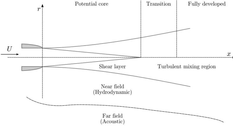
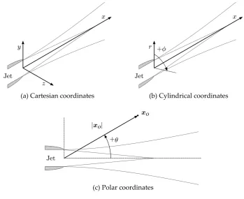
Figure 2.1shows the structure of a typical turbulent jet and the classification of its regions while figure 2.2 shows the sign convections used in jet aeroacoustics for

(34)

r

x Potential core Transition Fully developed

Near field (Hydrodynamic)

Far field (Acoustic)

Turbulent mixing region Shear layer

[image:34.595.89.491.94.311.2]

U

Figure 2.1: Turbulent jet schematic

(35)

x

y

z Jet

(a) Cartesian coordinates (b) Cylindrical coordinates

(c) Polar coordinates r

x

+Á

Jet

+_µ jx_o_j

x_o

[image:35.595.128.478.90.375.2]

Jet

Figure 2.2: Sign conventions for jet noise4

transition regionexists between the potential core and the fully developed region as the flow transitions to fully developed flow. The transition region is typically the area of greatest turbulence in the flow. Theturbulent mixing regionencompasses all of the flow where turbulent mixing takes place, including the shear layer.

Lighthill(1952) noted the primary term responsible for the amount of noise emitted by a jet isρ0U2, whereρ0 is the ambient fluid density. However, he also noted the effects of two important non-dimensional parameters, theMach number(M) and the Reynolds number(Re). The Mach number (M =U/c0) affects the efficiency of the noise sources, while the Reynolds number—since it represents the dominance of inertial over viscous fluid forces—affects the nature of the sound generation mechanisms. The Reynolds number for a circular jet is given by

Re= ρJUD µJ

, (2.3)

whereρJ is the fluid density at the jet exit,Dis the diameter of the jet, andµJ is the dynamic viscosity of the fluid at the jet exit. The Reynolds number is important for comparing jets of different sizes and velocities. It is especially useful for comparing

4_{Many experimental studies measure}

θfrom the upstream axis as opposed to the downstream axis,

(36)

small model jets to full-scale jets.

The demarcation between the near-field and far-field is not a well-defined physical location. In fact, tests with microphone measurements have shown that the dividing line is frequency dependent. Using the wavenumber5, k, which characterizes the spatial distribution of the sound waves, and the radial distance from the jet axis,r, Arndtet al.(1997) proposed a value ofkr=2 for the separation and reported a sharp divide between near-field and far-field behaviour at this location. It is clear that close to the jet, the dominant behaviour is hydrodynamic and far from the jet the dominant behaviour is acoustic. However, in the near field, even though acoustic fluctuations are masked by higher-intensity hydrodynamic fluctuations, they must be present because acoustic fluctuations start in the jet and propagate outward. In contrast to this, only acoustic behaviour is possible far from the jet because the medium is essentially quiescent far from the jet and no non-acoustic stress field associated with the jet can exist.

A further peculiarity of the noise emissions from turbulent jets is that the analysis of the emissions is a story of two different complexities. In the turbulent flow region, the fluctuations satisfy the full non-linear Navier–Stokes equations, numerical solutions of which are now possible in simple cases but not necessarily practical or informative for jet design. In the far field, the pressure fluctuations follow simple linear acoustics equations, which can be easily solved for given boundary conditions (typically a pressure distribution on a surface surrounding the turbulent flow). This reduced complexity of the far field gives hope to researchers that the acoustically important behaviour of jet turbulence can also be captured with a reduced-order model of the jet dynamics (Jordan & Colonius,2013). This observation forms the basis for the noise source modelling approach pursued inchapter 4.

2.2.4 Origins of jet noise research and the acoustic analogy

The advent of aeroacoustics research was the first part of the pioneering paper of Lighthill(1952), which addressed the production of sound by aerodynamic forces. He released a second part to the paper, which focused on turbulence as a sound source, two years later (Lighthill, 1954). In the first part of the paper,Lighthill introduced what became known as the ‘acoustic analogy.’ Lighthill’s novel idea was to take the Navier–Stokes equations6_{, which govern fluid motion, and to rearrange them}

5_k₌₂

π/λ, whereλis the wavelength of the sound waves.

6_{Although the Navier–Stokes equation is the name of the momentum conservation equation for a}

(37)

into a general form of the wave equation. In this way, he separated the terms in the equations of motion into those satisfying the wave equation, which represent the observed sound field in a quiescent medium, from all the other terms. All the other terms were collapsed into an externally applied stress field. Setting mass sources and external forces to zero, Lighthill(1952) rearranged the Navier–Stokes equations to obtain7

∂2ρ0

∂t2 −c 2 0

∂2ρ0

∂x2_i

= ∂

2_T ij

∂xi∂xj

, (2.4)

whereTij is the instantaneous applied stress at any point. Tij has become known as the Lighthill stress tensor and is given by8

Tij = ρuiuj+σij−c20ρδij, (2.5)

where δij is the Kronecker delta function andσij is the full stress tensor at the location of the fluid element. Physically, this means that the sound generation and propagation from an arbitrary fluid motion is equivalent to a distribution of appropriate sources. All of these sources are contained in the Lighthill stress tensor. In his own words, Lighthill describedTij in the following way:

The external stress system Tij incorporates not only the generation of sound, but its convection with the flow (in part of the term ρuiuj), its propagation with variable speed and gradual dissipation by conduction (each in part of the difference between pressure variations andc2₀times the density variations), and its gradual dissipation by viscosity (in the viscous contribution to the stress systemσij) (Lighthill,1952)9.

In practice, this means that an appropriate model for the Lighthill stress tensor is all that is required to predict the sound field generated by an arbitrary fluid flow. It is important to note that this form of the acoustic analogy contains no approximations; it is exactly equivalent to the original equations of motion. In itself, the analogy is not particularly useful in simplifying the problem of jet noise prediction since calculating the Lighthill stress tensor directly is no easier than solving the original equations of motion; however, the knowledge that the acoustic field of any arbitrary fluid motion is equivalent to a field of appropriate sources is powerful. Lighthill’s acoustic analogy

7_{Apart from changing the acoustic variable from}_p_to

ρ, the major difference betweenequation (2.1)

andequation (2.4)is the addition of the source term to the right hand side. Aeroacoustics can be defined as the study of flows in which the sound source is this term on the right hand side ofequation (2.4) (Hirschberg,2001).

8_{An alternative formulation for the Lighthill stress tensor can be written in terms of the viscous stress}

tensor asTij=ρuiuj+δij p+ρc2₀−τij.

9_{The notation used in this quotation has been changed slightly from the original paper in order to}

(38)

provides a starting point for making approximations to the Lighthill stress tensor, which can simplify the problem of jet noise prediction considerably (Hirschberg,2001). The first of these approximations was carried out byLighthillin the same paper. He first argued that the viscosity terms of the stress tensor should be ignored, and he added that for flows at low Mach number (M=U/c0) , where the flow is nearly isothermal, the final term is also largely cancelled by the pressure in the stress tensor. His simplifications led toTij ≈ρ0uiuj(Goldstein,1974). Theρuiujterms are referred to as the Reynolds stresses, which are considered to beρ0uiuj when density fluctuations are neglected. This leads to the conclusion that the Reynolds stresses are the main sources of sound for these flows. Applying this simplification to jets led directly to several scaling laws between observed sound power and characteristics of the jet. The most important of these is the eighth-power scaling law, which states that the observed sound power scales withU8. This meant that noise could be reduced simply by increasing the diameter of the engine and reducing the jet velocity for the same total thrust output. This improvement was also amplified by the introduction of high-bypass engines. The bypass ratio is the ratio of air flowing into the engine bypassing the engine core to the air flowing through the engine core, so increasing bypass ratio typically increases jet diameter. High-bypass engines not only produce less noise for a given thrust output, but are also more fuel efficient. In fact, high-bypass engines were developed primarily for their fuel efficiency. An additional advantage of high-bypass engines is that the flow bypassing the combustor also partially buffers the more turbulent, sound-producing flow behind the combustor. These advances led to significant jet noise reductions for aircraft since the 1950s (Morris & Viswanathan, 2011). Lighthill’s purely theoretical scaling law has been verified experimentally with impressive agreement. It has also led to the development of semi-empirical models to predict jet noise for well-established jet geometries (Self,2004).

2.2.5 Qualitative properties of jet noise

2.2.5.1 Directivity

Early jet noise measurements quickly indicated that the jet noise emissions were not uniform at all angles of the jet. In fact, Lighthill’s original paper argued that the increased sound intensity measured could be accounted for by considering the sources to be moving eddies (Lighthill, 1952). Ffowcs Williams (1963) expanded this idea by modelling the noise sources as acoustic quadrupoles convecting at high speed in the jet. In his work, Ffowcs Williams (1963) used a modified conclusion from Lighthill that the intensity of the sound varied with|1−Mccosθ|−5—where

(39)

of the convecting source—to conclude that for very high-speed jets (Mc > 1) the sound power scaled withU3. This result also agreed with many experiments of the time that were indicating thatU8 scaling seemed too high for very high-speed jets. The important result for the directivity suggested by these authors was the direction intensity factor|1−Mccosθ|−5, which gave a basis for understanding the variation of

jet noise at different angles. This result became known as ’convective amplification’ and is postulated to result from the fact that convection makes cancellation of quadrupole sources less effective, increasing their efficiency (Crighton,1975). However, evidence for convective amplification is not fully accepted (Crighton,1975;Morris & Boluriaan, 2004).

Ffowcs Williams(1963) also noted that observed frequencies should be compared at various observer locations only after shifting the sound spectrum by a Doppler factor of (1−Mccosθ). An important thing to note with these factors, is that for

θ =90◦, both the amplification and the Doppler factor are unity. This indicates that

for measurements at 90◦, no corrections are necessary. For this reason, 90◦ is often used as the reference point for theoretical models, especially semi-empirical models. These results imply only one source of jet noise, of which the observed directivity is an inherent property. However, the predictions of this method do not always line up with experimental measurements. An additionally compounding factor is that noise directivity relations have also been observed to vary with the frequency of noise considered.

2.2.5.2 Mach number effects

(40)

for supersonic jets by operating a converging-diverging nozzle at design conditions. However, this is typically unfeasible in practice. As this work is focused on subsonic jets, only jet mixing noise will be considered.

Apart from these additional noise sources, the Mach number also affects the characteristics of jet mixing noise. Lighthill’s original theory led to the result that not only was there more energy in high-speed flows available to be transformed into acoustic energy, but also the conversion became more efficient as the Mach number increased. This helps account for the high exponent in the eighth-power law. The correction introduced byFfowcs Williams(1963) was related to an assumption that the sources of jet noise were of finite extent, which partly reduced the exponent for his third-power scaling law. For subsonic jets, the main effect of the Mach number is simply this scaling, with only small changes to the shape of the noise spectra. This result is presented, for example, byViswanathan(2004).

2.2.5.3 Temperature effects

Most jet engines operate at relatively high temperatures due to the combustion of fuel as the power source. For high-bypass engines there is also a large temperature difference between the combustor flow and the bypass flow. Large variations in temperature change the properties of the fluid travelling through the engine and thus have a marked effect on jet noise. Extensive experiments have been carried out to test the effect of temperature on jet noise emissions (Tanna et al.,1975;Viswanathan, 2004). The effect of temperature is not straightforward. The prevailing result is that for low-speed jets, an increased temperature ratio10 increases noise, while for high-speed jets it decreases noise. The transition between the two regimes has been shown to be close to M=0.8 (Viswanathan,2004). Viswanathan(2006) proposed a set of scaling laws for which the exponent was a function of temperature ratio. Of course, for an unheated jet (TJ/T0=1) at low Mach number, the result was equivalent to Lighthill’s eighth-power scaling law.Viswanathan(2004) also noted similarities in the spectral shape of noise emissions for lowθ between unheated low subsonic jets and highly

heated supersonic jets. However, the full effects of temperature on jet noise are still a subject of intense debate.

2.2.5.4 Sound propagation

Part of the difficulty in understanding where jet noise originates in the jet is associated with the effect of the jet flow on the propagation of sound. In a stagnant medium,

10_{The temperature ratio,} _T

(41)

r

x U

Mean flow profile Cone of silence Sound source

[image:41.595.101.508.93.279.2]

Radiated sound

Figure 2.3: Sound propagation through a mean jet flow profile

sound propagates outward evenly in all directions. In a homogeneous two-dimensional mean flow, the difference in velocity—and possibly temperature and density—between adjacent locations causes the sound rays to bend. When the properties of the medium also vary, the sound waves can speed up and slow down according to the local speed of sound, as well as bend and shift according to disturbances in fluid motion. A true prediction of sound propagation in turbulent flow can only be obtained by solving for the turbulent flow field, which is currently impossible for practical flows. Since the sound signals observed from jet noise emissions have fairly constant directionality, there is hope that reasonable estimates of sound propagation can be obtained from mean flow profiles.

The effect of sound refraction in a mean flow is illustrated infigure 2.3. As a wave front propagates in the direction of flow. The velocity difference across the wave front causes the wave to turn outwards. This effect is reversed for wave fronts propagating upstream. This causes a region of reduced sound intensity at emission angles close to the downstream axis known as thecone of silence, which is also illustrated infigure 2.3. The reduction in intensity has been observed to be as great as 20 dB byAtvars et al.

(1966).

(42)

2.3 Historical developments in jet noise research

2.3.1 Extended acoustic analogies

ThoughLighthill’s (1952) acoustic analogy, described byequation (2.4), was the first re-casting of the governing equations of fluid dynamics into a wave equation, it is not the only possible formulation. Acoustic analogies are usually developed in the form

L[ρ] |{z} Propagation

= Q

|{z} Source

, (2.6)

where L[·]is the propagation operator andQis the source term. InLighthill’s (1952) analogy, the propagation operator is the wave equation in a quiescent medium, and the source is all the other terms in the Navier–Stokes equations. This is the simplest possible formulation for the propagation operator, with the most complicated form for the source term. The benefits of putting more flow physics into the propagation term (left-hand side) is that the source term becomes simpler—making it easier to model—and that the physics of the sound propagation are separated from the physics of the sound generation, allowing a better understanding of what the ‘true’ source is. However, the disadvantage is the added complexity of solving the equation. While Lighthill’s (1952) propagation problem can be solved with a simple free-space Green’s function, more complicated forms of the source are not as easy to solve. In the extreme case, where all the physics are placed on the left-hand side, the equations become the same as the Navier–Stokes equations, completely cancelling the advantage of using an acoustic analogy at all.

Lilley(1973) was one of the first to incorporate more flow physics in the propa-gation term. He incorporated the effect of mean flow refraction (see§ 2.2.5.4) into the propagation term by using the Linearized Euler Equations as the wave operator where the equations were linearized about the mean flow of the jet. Lilley’s approach was well-received and many subsequent authors expanded on his ideas (Lilley,1991; Tam,1998). Over the years, several other variations have been proposed to incorporate various other effects, for example, inGoldstein (2003,2001) andPhillips(1960). The basic results of these studies have primarily been a greater understanding of jet noise and propagation, but accurate noise predictions based on these techniques that apply to wide ranges of operating conditions and emission directions are still rare (Morris & Viswanathan,2011).

(43)

2.3. HISTORICAL DEVELOPMENTS IN JET NOISE RESEARCH

part of the propagation term, allowing specific components of the jet noise problem to be considered in each case.

2.3.2 Large-scale and fine-scale noise sources

The earliest understanding of turbulence was as a superposition of uncorrelated random eddies. In the early 1960s, evidence for larger-scale structures began to accumulate. A fuller discussion of the role of large-scale structures in jet noise and the historical developments in their understanding is reserved forchapter 4, in which the role one type of large-scale structure is the focus. However, for the current discussion, it is only necessary to introduce the conceptual separation of large-scale and small-scale turbulence structures.

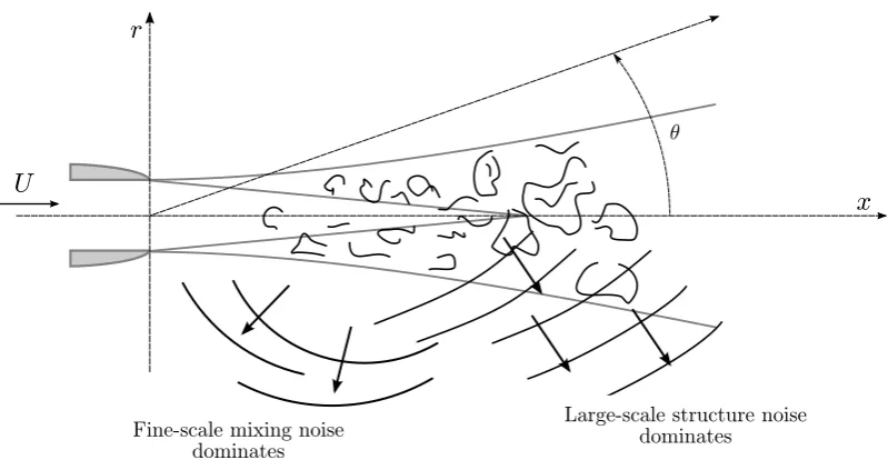
Unhappy with the poor agreement between the prediction methods of the time, and after analyzing a large experimental database,Tamet al.(1996) proposed a division of jet noise into two independent sources. The first source is said to be attributed to the fine-scale structures of the turbulence while the second is associated with the large-scale structures. Corresponding to these sources,Tamet al.(1996) introduced two ‘similarity spectra,’ which are said to be universal for axisymmetric jets. These spectra are termed the Fine-Scale Similarity (FSS) spectrum and the Large-Scale Similarity (LSS) spectrum, respectively. The FSS spectrum seems to characterize the observed emission spectrum of high observer angles (θ &80◦) while the LSS spectrum

characterizes the spectrum at low observer angles (θ .40◦, Tam,1998). Figure 2.4

shows this effect schematically. Despite the compelling experimental evidence for the view proposed by Tam et al., no consensus has been reached as to whether a two-source paradigm of jet noise better reflects the sound generation mechanics than the traditional one-source paradigm.

The shortcoming of the FSS and LSS approach to jet noise prediction is that the scheme lacks predictive power because it is predominantly empirical. Ultimately, the similarity spectra are fitted to experimental data after experimental testing, which means that the model always involves arbitrary constants that are not easy to predict in advance. Also, though the database used by Tam et al. (1996) to generate the similarity spectra represents the mechanics of simple circular jets, novel designs that deviate from simple jets cannot necessarily be expected to follow the same trends. The advantage of the approach is the effectiveness with which it explains the seemingly universal characteristics of the noise emissions from circular jets.

(44)

r

x U

Fine-scale mixing noise dominates

Large-scale structure noise dominates

[image:44.595.93.493.87.294.2]

µ

Figure 2.4: Theorized noise components of a jet. Adapted fromTamet al.(2008).

important consideration is that significant noise reductions based on noise reduction technologies are more feasible if large-scale structures are the dominant sound source. For example, if the dominant sound source is random turbulent fluctuations evenly distributed everywhere in the jet, the likelihood that a device could be designed to exert significant control authority over all locations at once is quite small. However, if the dominant source is a large fluctuation correlated over a significant portion of the length of the jet, it could more easily be influenced by a device that acts at one specific location, which is a more feasible design goal. Therefore, the discovery of the importance of large-scale structures in jet noise is a promising development in the pursuit of practical jet noise reduction schemes.

2.4 Noise reduction technologies

2.4.1 Introduction

(45)

2.4. NOISE REDUCTION TECHNOLOGIES

at the model scale may have no effect or even detrimental effects on full-scale jets. Another issue is that while some of these techniques may be effective at one set of flight conditions, at different periods during flight they may have negligible or negative effects. Nevertheless, advances have been made and some examples of the major technologies are discussed here.

There are two main categories for noise reduction technologies: passive control andactive control. Passive control is the traditional approach to jet noise reduction. It utilizes time-invariant design changes, such as fixed flow control devices and jet geometry modifications, which attempt to influence the mean statistics of the turbulence or control the growth of the shear layer, for example. Modern techniques have begun to employ active control, incorporating time-varying influences on the jet flow to target specific flow phenomena, such as those associated with dominant peak frequencies in the jet noise spectrum.

2.4.2 Passive control

The best example of a passive control technique that has led to significant noise reductions is the introduction of the high-bypass turbofan engine described in§ 2.2.4. The reduction arises from the decrease in exhaust speed for a given thrust requirement when the jet diameter is increased, which reduces noise according toLighthill’s (1952) eighth-power scaling law. This is a rare example of where aeroacoustic and aerody-namic performance were both improved with a single design change. However, there are both theoretical and practical limits to the possible increase of the diameter of a turbofan engine. Ffowcs Williams & Gordon(1965) noted that as the exhaust speed decreases, an additional source of noise appears, which is normally concealed by jet noise and in addition to other typically observed noise components. Jet engines can also not be made arbitrarily large because of the practical limitations of manufacturing fan and turbine blades of sufficient size and strength.

(46)

may be a more important design consideration than noise reductions. The effect of chevrons is generally a reduction in low-frequency noise with an accompanying increase in high-frequency noise, but the overall impact is usually positive. The parameters for chevron nozzle design include chevron number, length, penetration, and asymmetry. Parametric testing has been carried out byBridges & Brown(2004), who concluded that the relationships between these parameters are complex but that trends are apparent. Flight tests have yielded promising results and now Boeing has even included chevrons in the design of its recently released 787 (Herkeset al.,2006). A database of information on the effects of chevrons has been growing (Bridges,2002; Kennedy,2010), recording the effect of chevrons on the hydrodynamic field of the jet both from the perspective of flow statistics (Kennedy,2010) and in a time-resolved full-field manner (Scaranoet al.,2010), but aside from the concept of ‘enhanced’ mixing, their true mechanism of noise reduction is yet to be clearly understood.

Passive control techniques suffer from the inability to respond to different perfor-mance requirements at different stages in flight. For example, noise reductions are most important at takeoff when the engines are at full power and regulatory noise limits are in place. At cruise, thrust penalties are more important since there are no ground-based observers affected by the aircraft’s noise emissions. Additionally, while mixing devices can often be tuned to reduce noise at some flight conditions, they may actually increase noise at different conditions, limiting their effectiveness.

2.4.3 Active control

Broadly speaking, active control techniques are those that require a power source to operate, and can therefore be activated, deactivated, or modified during aircraft operation. Some passive controllers have active analogues. For example, an alternative to physical nozzle inserts isfluidic nozzle inserts(Powerset al.,2013), and an alternative to chevrons isfluidic chevrons(alsomicrojetsorfluidevrons;Henderson,2009;Laurendeau

et al.,2008;Martens & Haber,2008). Both systems seek to reproduce the advantages of their passive counterparts while obtaining the benefits of active control by injecting fluid into the jet stream, affecting the momentum of the mixing region in a similar way to their passive counterparts. The principal advantage of these systems is that they can be deactivated when unnecessary or adjusted for different flight conditions, reducing potential aerodynamic performance penalties when noise reductions are less important.

(47)

2.5. CONCLUSION

allows, for example, forcing of the jet at various frequencies (Mauryet al.,2011,2012), or unsteady forcing caused by steady rotation of a microjet (Kœniget al.,2011,2013) either of which can influence the jet noise emissions. Though these types of devices can be tuned to cause noise reductions under certain flight conditions, they areopen-loop controllers; that is, they do not use feedback from the system to control their operation. The newest generation of development in active jet noise control is currently pursuing the use ofclosed-loop controllers, which use real-time measurements obtained during operation coupled with dynamic models of the jet mechanics to detect and influence ‘noisy’ structures (Jordan & Colonius,2013).

In order to implement these types of controllers, it is necessary to have an un-derstanding of the noise source mechanics that can predict both the statistical and time-domain noise emissions. Such a technique is developed in chapter 4while a time-domain error metric—necessary to implement traditional closed-loop control schemes—is developed inchapter 5.

Non-periodic unsteady forcing suitable for use in closed-loop control can be achieved by employing actuators with a faster response time, such as plasma actuators (Kastneret al.,2006;Samimyet al.,2004). Though closed-loop active control of jet noise may never be feasible on a production aircraft, the insight gained from a successful application in a lab setting would be a boon to the understanding of jet noise sources. Regardless of the effectiveness of a closed-loop control system to reduce the total noise level for regulatory purposes, if a control system coupled with a suitable dynamic exerted significant control authority over the jet noise emissions, it would greatly increase the aeroacoustics community’s understanding of jet noise source mechanics.

2.5 Conclusion

Over sixty years afterLighthill(1952) laid the foundations of aeroacoustics, research in the field is as active as ever. Each new development leads to more questions surrounding the nature of jet noise sources and potential techniques to mitigate jet noise emissions.

(48)

obtained only indirectly with other jet design innovations (e.g.high-bypass engines) or at the expense of large experimental campaigns and many years of testing. Even a technology as simple as chevron nozzles has taken decades to finally be incorporated into production jets, and the contribution of chevrons to noise reductions is moderate. Today, the aeroacoustics community broadly understands the salient features of jet noise, and many of its characteristics have been well documented. However, modern noise prediction techniques still lack the predictive power necessary to incorporate noise concerns into the aircraft design cycle, and design changes still require significant testing before they can be shown to be beneficial. Practical jet noise reductions are as important as ever because the continued expansion of the airline industry—seeking to connect more people and places around the world—is accompanied by continued growth in community opposition concerned with the negative effects of jet noise.

(49)

Chapter 3

Source analysis using time-resolved

Particle Image Velocimetry

3.1 Introduction

(50)

measurements (Papamoschou et al., 2010) and to data from numerical simulations (Bogey & Bailly,2007).

The introduction of Particle Image Velocimetry (PIV, see § 3.2.2) for spatially resolved flow measurements has largely revolutionized the acquisition of data from flow experiments (Raffel et al., 2007), allowing large flow fields to be measured simultaneously. Perhaps the bright future for PIV is best indicated by the rapid extension of the technique to fully volumetric, three-component velocity measurements by a variety of techniques (Elsingaet al.,2006;Hinsch,1995). These techniques have even been applied to transitional jets to consider the development of flow structures (Violato & Scarano,2011). A fullness of flow information is now available that likely could never have been imagined by early aeroacoustics researchers. Until recently, this extensive spatial information has been obtained at the expense of time-domain resolution with maximum PIV acquisition rates reaching only a few frames per second.

The advent of Digital PIV (Willert & Gharib,1991) started a rapid escalation toward higher acquisition rates, and recent developments in laser and camera technology have led to the introduction of Time-Resolved PIV (TR-PIV, see§ 3.2.3), where the acquisition rate is high enough to temporally resolve the flow field. The acquisition rate necessary to resolve a particular flow is dependent on the time scales of the events to be resolved, and for turbulence, the required acquisition rates are very high. Current equipment in common use is limited to acquisition rates around 10 kHz, while some limited tests have been carried out as high as 25 kHz (Bridges & Wernet,2007;Wernet, 2007b) with reduced Fields Of View (FOVs). These increased acquisition rates, as well as creative applications of low-speed PIV equipment have led to a number of PIV investigations of aeroacoustic flows (Morris,2011;Schröderet al.,2004;Seiner,1998). Despite these high data rates, the discrete nature of PIV measurements introduces the problem of temporal aliasing because the measurement of the flow velocity and the discrete sampling cannot be separated. This is because the PIV algorithm works by comparing two discrete images so there is no continuous signal to which an anti-aliasing filter can be applied. This anti-aliasing of high-frequency information into lower frequencies limits the accuracy of TR-PIV measurements in the frequency domain. This aliasing effect has been noted by previous investigators (Bridges & Wernet,2007; Wernet,2007b), although its effect on the determination of the space–time correlation, Ru0_p0(x_s,x_o,_τ), and the frequency-domain equivalents has not been investigated.

(51)

3.1. INTRODUCTION

and TR-PIV offers no direct benefits. Traditional PIV has been used byHenninget al.

(2008,2010a,b) in a number of flow configurations including a cylinder in cross-flow and a cold jet. This was achieved by coupling 5000 PIV measurements with a long series of high sample rate microphone measurements lasting over 30 minutes. In fact,§ 3.5.2describes how the traditional PIV approach is superior to TR-PIV when considering the contribution of each velocity measurement to the statistical significance of the correlation estimate. However, because correlation is ambiguous in the direction of causation, it is often necessary to observe the full development of a fluctuation in real time to determine how it originated and became an efficient sound emitter. TR-PIV’s ability to record individual flow realizations enables a connection to be made between the development of each flow fluctuation and its contribution to the flow statistics, which may not be apparent in the averaged flow development animated by mapping the correlation coefficient. From a control perspective, this translates to a more concrete ability to see what fluid events caused a fluctuation, making it possible to propose schemes to counteract that source activity. The calculation of frequency-domain statistics such as coherence also provides another useful perspective in source analysis. Specifically, the calculation of the coherence is the first step toward the application of multiple input/output source identification analysis (Fitzpatrick & Rice,1988). Also, since the introduction of TR-PIV-based time-domain sound field prediction techniques (Haigermoser, 2009; Koschatzky et al., 2011), comparison of the correlation and coherence features between the measured flow and the measured and predicted sound fields may yield useful insight. In the present thesis, however, since this work represents the first step toward using TR-PIV-based correlation in these applications, the discussion is limited to the ability of TR-PIV to reproduce the space–time correlation value,Ru0_p0(x_s,x_o,τ), and the space–frequency coherence,

γ2_u0_p0(xs,xo,f).