www.hydrol-earth-syst-sci.net/19/3557/2015/ doi:10.5194/hess-19-3557-2015
© Author(s) 2015. CC Attribution 3.0 License.
Improving multi-objective reservoir operation optimization with
sensitivity-informed dimension reduction
J. Chu1, C. Zhang1, G. Fu2, Y. Li1, and H. Zhou1
1School of Hydraulic Engineering, Dalian University of Technology, Dalian 116024, China 2Centre for Water Systems, College of Engineering, Mathematics and Physical Sciences, University of Exeter, North Park Road, Harrison Building, Exeter EX4 4QF, UK
Correspondence to: C. Zhang ([email protected])
Received: 10 March 2015 – Published in Hydrol. Earth Syst. Sci. Discuss.: 8 April 2015 Revised: 25 June 2015 – Accepted: 31 July 2015 – Published: 12 August 2015
Abstract. This study investigates the effectiveness of a sensitivity-informed method for multi-objective operation of reservoir systems, which uses global sensitivity analysis as a screening tool to reduce computational demands. Sobol’s method is used to screen insensitive decision variables and guide the formulation of the optimization problems with a significantly reduced number of decision variables. This sensitivity-informed method dramatically reduces the com-putational demands required for attaining high-quality ap-proximations of optimal trade-off relationships between con-flicting design objectives. The search results obtained from the reduced complexity multi-objective reservoir operation problems are then used to pre-condition the full search of the original optimization problem. In two case studies, the Dahuofang reservoir and the inter-basin multi-reservoir sys-tem in Liaoning province, China, sensitivity analysis results show that reservoir performance is strongly controlled by a small proportion of decision variables. Sensitivity-informed dimension reduction and pre-conditioning are evaluated in their ability to improve the efficiency and effectiveness of multi-objective evolutionary optimization. Overall, this study illustrates the efficiency and effectiveness of the sensitivity-informed method and the use of global sensitivity analysis to inform dimension reduction of optimization problems when solving complex multi-objective reservoir operation prob-lems.
1 Introduction
Reservoirs are often operated considering a number of con-flicting objectives (such as different water uses) related to environmental, economic, and public services. The optimiza-tion of the reservoir operaoptimiza-tion system (ROS) has attracted substantial attention over the past several decades. In China and many other countries, reservoirs are operated according to reservoir operation rule curves which are established at the planning/design stage to provide long-term operation guilines for reservoir management to meet expected water de-mands. Reservoir operation rule curves usually consist of a series of storage volumes or levels at different periods (Liu et al., 2011a, b).
Si-monovic, 1992; Wurbs, 1993; Teegavarapu and SiSi-monovic, 2001; Labadie, 2004).
In a different way, PSO predefines a rule curve shape and then utilizes optimization algorithms to obtain the combina-tion of rule curve parameters that provides the best reser-voir operating performance under possible inflow scenarios or a long inflow series (Nalbantis and Koutsoyiannis, 1997; Oliveira and Loucks, 1997). In this way, most stochastic as-pects of the problem, including spatial and temporal corre-lations of unregulated inflows, are implicitly included, and reservoir rule curves could be derived directly with genetic algorithms and other direct search methods (Koutsoyiannis and Economou, 2003; Labadie, 2004). Because PSO reduces the curse of dimensionality problem in ISO and ESO, it is widely used in reservoir operation optimization (Chen, 2003; Chang et al., 2005; Momtahen and Dariane, 2007). In this study, the PSO-based approach is used to solve the ROS problem.
In the PSO procedure to solve the ROS problem, the val-ues of storage volumes or levels in reservoir operation rule curves are optimized to achieve one or more objectives di-rectly. Quite often, there are multiple curves, related to dif-ferent purposes of reservoir operation. The dimension of a ROS problem depends on the number of the curves and the number of time periods. For a cascaded reservoir system, the dimension can be very large, which increases the complexity and problem difficulty and poses a significant challenge for most search tools currently available (Labadie, 2004; Draper and Lund, 2004; Sadegh et al., 2010; Zhao et al., 2014).
In the context of multi-objective optimal operation of a ROS, there is not one single operating policy that im-proves simultaneously all the objectives and a set of non-dominating Pareto-optimal solutions are normally obtained. The traditional approach to multi-objective optimal reservoir operation is to reformulate the multi-objective problem as a single-objective problem through the use of some scalariza-tion methods, such as the weighted sum method (Tu et al., 2003, 2008; Shiau, 2011). This method has been developed to repeatedly solve the single-objective problem using differ-ent sets of weights so that a set of Pareto-optimal solutions to the original multi-objective problem could be obtained (Srinivasan and Philipose, 1998; Shiau and Lee, 2005). An-other well-known method is the ε-constraint method (Ko et al., 1997; Mousavi and Ramamurthy, 2000; Shirangi et al., 2008): all the objectives but one are converted into con-straints and the level of satisfaction of the concon-straints is op-timized to obtain a set of Pareto-optimal solutions. However, with the increase in problem complexity (i.e., the number of objectives or decision variables), both approaches become in-efficient and ineffective in deriving the Pareto-optimal solu-tions.
In the last several decades, bio-inspired algorithms and tools have been developed to directly solve multi-objective optimization problems by simultaneously handling all the objectives (Nicklow et al., 2010). In particular,
multi-objective evolutionary algorithms (MOEAs) have been in-creasingly applied to the optimal reservoir operation prob-lems, with the intent of revealing trade-off relationships be-tween conflicting objectives. Suen and Eheart (2006) used the non-dominated sorting genetic algorithm (NSGAII) to find the Pareto set of operating rules that provides decision makers with the optimal trade-off between human demands and ecological flow requirements. H. F. Zhang et al. (2013) used a multi-objective adaptive differential evolution com-bined with chaotic neural networks to provide optimal trade-offs for multi-objective long-term reservoir operation prob-lems, balancing hydro-power operation and the requirement of a reservoir ecological environment. Chang et al. (2013) used an adjustable particle swarm optimization – genetic al-gorithm hybrid alal-gorithm to minimize water shortages and maximize hydro-power production in management of Tao River water resources.
2 Problem formulation
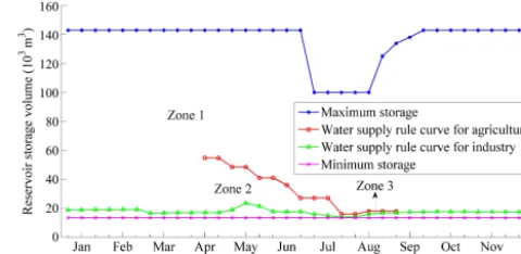
Most reservoirs in China are operated according to rule curves, i.e., reservoir water supply operation rule curves. Since they are based on actual water storage volumes, they are simple to use. Figure 1 shows an illustration of rule curves for Dahuofang reservoir based on 36 10-day periods.
As we know, water demand can be fully satisfied only when there is sufficient water in the reservoir. The water sup-ply operation rule curve, which is used to operate most reser-voirs in China, represents the limited storage volume for wa-ter supply in each period of a year. In detail, wawa-ter demand will be fully satisfied when the reservoir storage volume is higher than the water supply operation rule curve; conversely, water demand needs to be rationed when the reservoir storage volume is lower than the water supply operation rule curve. In general, a reservoir has more than one water supply tar-get, and there is one to one correspondence between water supply rule curve and water supply target. The water supply with lower priority will be limited prior to the water sup-ply with higher priority when the reservoir storage volume is not sufficient. To reflect the phenomenon that different wa-ter demands can have different reliability requirements and thus different levels of priority in practice, the operation rule curve for the water supply with the lower priority is located above the operation rule curve for the water supply with the higher priority.
Figure 1 shows water supply operation rule curves for agri-culture and industry where the maximum storage is smaller in the middle due to the flood control requirements in wet seasons. In Fig. 1, the red line with circles represents the water supply rule curve for agriculture, the green line with triangles represents the water supply rule curve for industry. The water supply rule curve for agriculture with lower prior-ity is located above the water supply rule curve for industry with higher priority. The water storage available between the minimum and maximum storages is divided into three parts: zone 1, zone 2, and zone 3 by the water supply rule curves for agriculture and industry.
[image:3.612.308.548.68.185.2]Specifically, both the agricultural demandD1and the in-dustrial demandD2could be fully satisfied when the actual water storage is in zone 1, which is above the water supply rule curve for agriculture. When the actual water storage is in zone 2, the industrial demand could be fully satisfied, and the agricultural demand has to be rationed. Both the agricultural demand and the industrial demand have to be rationed when the actual water storage is in zone 3. The water supply rule for a specific water user consists of one water supply rule curve and rationing factors that indicate the reliability and priority of the water user. The rationing factors used to deter-mine the amount of water supply for different water demands can be either assigned according to the experts’ knowledge or determined by optimization (Shih and ReVelle, 1995). In this paper, rationing factors are given at the reservoir’s design stage according to the tolerable elastic range of each water
Figure 1. Reservoir operational rule curves.
user in which the damage caused by rationing water supply is limited. Assuming that the specified water rationing factor
α1 is applied to the water supply rule curve for agriculture in Fig. 1, the agricultural demandD1could be fully supplied without rationing when the actual water storage is in zone 1; however, when the water storage is in zone 2 or zone 3, the agricultural demand has to be rationed, i.e.,α1×D1. Simi-larly, assuming that the specified water rationing factorα2is applied to the water supply rule curve for industry in Fig. 1, the industrial demandD2could be fully supplied without ra-tioning when the actual water storage is in zone 1 or zone 2; however, when the water storage is in zone 3, the industrial demand has to be rationed, i.e.,α2×D2.
To provide long-term operation guidelines for reservoir management for meeting expected water demands for fu-ture planning years, the projected water demands and long-term historical inflow are used. The optimization objective for water supply operation rule curves is to minimize water shortages during the long-term historical period. The ROS design problem is formulated as a multi-objective optimiza-tion problem, i.e., minimizing multiple objectives simultane-ously. In this paper, the objectives are to minimize industry and agriculture water shortages:
minfi(x)=SIi= 100
N N X
j=1 D
i,j−Wi,j(x) Di,j
2
, (1)
wherex is the vector of decision variables, i.e., the water storages at different periods on a water supply rule curve; SIi is the shortage index for water demandi(agricultural water demand wheni=1, industrial water demand wheni=2), which measures the average annual shortage occurred during
N years, and is used as an indicator to reflect water supply efficiency; N is the total number of years simulated; Di,j is the demand for water demandiduring thejth year; and
rationed,D1,t. If the actual water storage is below the water supply rule curve for agricultural water demand at periodt, the delivered water for agricultural water demand at periodt
is its rationed demands,α1×D1,t.
For the ROS optimization problem, the mass balance equa-tions are
St+1−St=It−Rt−SUt−Et, (2)
Rt=g (x) , SUt=k (x) , Et=e (x) , (3)
STmint ≤St ≤STtmax, STmint ≤x≤STmaxt , (4) whereStis the initial water storage at the beginning of period t;St+1is the ending water storage at the end of periodt;It, Rt, SUt, andEt are inflow, delivery for water use, spill and evapotranspiration loss, respectively; and STmaxt and STmint are the maximum and minimum storage, respectively. Addi-tionally, becauseWi,j(x)in Eq. (1) is the actually delivered water for water demandiduring thejth year,Rin that year is equal to the sum:W1,j(x)+W2,j(x).
3 Methodology
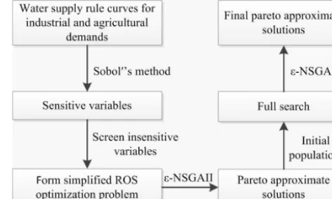
Pre-conditioning is a technique that uses a set of known good solutions as starting points to improve the search process of optimization problems (Nicklow et al., 2010). It is very challenging to determine good initial solutions, and differ-ent techniques including the domain knowledge can be used. This study utilizes a sensitivity-informed dimension reduc-tion to develop simpler search problems that consider only a small number of highly sensitive decisions. The results from these simplified search problems can be used to successively pre-condition the search for larger, more complex formula-tions of ROS design problems. The ε-NSGAII, a popular multi-objective evolutionary algorithm, is chosen as it has been shown to be effective for many engineering optimiza-tion problems (Kollat and Reed, 2006; Tang et al., 2006; Kollat and Reed, 2007). For the two objectives considered in this paper, their epsilon values inε-NSGAII (εSI1 andεSI2) were chosen based on reasonable and practical requirements and were both set to 0.01. According to the study by Fu et al. (2012), the sensitivity-informed methodology, as shown in Fig. 2, has the following steps:
1. Perform a sensitivity analysis using Sobol’s method to calculate the sensitivity indices of all decision variables regarding the ROS performance measure.
2. Define a simplified problem that considers only the most sensitive decision variables by imposing a user specified threshold (or classification) of sensitivity. 3. Solve the simplified problem using ε-NSGAII with a
small number of model simulations.
[image:4.612.310.547.69.211.2]4. Solve the original problem using ε-NSGAII with the Pareto-optimal solutions from the simplified problem fed into the initial population.
Figure 2. Flowchart of the sensitivity-informed methodology.
3.1 Sobol’s sensitivity analysis
Sobol’s method was chosen for sensitivity analysis because it can provide a detailed description of how individual variables and their interactions impact model performance (Tang et al., 2007b; C. Zhang et al., 2013). A model could be represented in the following functional form:
y=f (x)=f x1,· · ·, xp, (5) wherey is the goodness-of-fit metric of model output, and x= x1,· · ·, xp is the parameter set. Sobol’s method is a variance-based method, in which the total variance of model output,D (y), is decomposed into component variances from individual variables and their interactions:
D (y)=X
i
Di+
X
i<j Dij+
X
i<j <k
Dij k+ · · · +D12···m, (6)
whereDi is the amount of variance due to theith variablexi, andDij is the amount of variance from the interaction be-tweenxi andxj. The model sensitivity resulting from each variable can be measured using the Sobol’s sensitivity in-dices of different orders:
First-order index: Si= Di
D, (7)
Second-order index: Sij= Dij
D , (8)
Total-order index: ST i=1− D∼i
D , (9)
whereD∼i is the amount of variance from all the variables except forxi, the first-order indexSimeasures the sensitivity from the main effect ofxi, the second-order indexSij mea-sures the sensitivity resulting from the interactions between
xi andxj, and the total-order indexST i represents the main effect ofxiand its interactions with all the other variables. 3.2 Performance metrics
Table 1. Reservoir characteristics and yearly average inflow (106m3).
Reservoir Minimum Utilizable Flood control Yearly average name capacity capacity capacity inflow
Dahuofang 134 1430 1000 1570
the approximation sets derived from replicate multi-objective evolutionary algorithm runs. Three indicators were selected: the generational distance (Veldhuizen and Lamont, 1998), the additiveε-indicator (Zitzler et al., 2003), and the hyper-volume indicator (Zitzler and Thiele, 1998).
The generational distance measures the average Euclidean distance from solutions in an approximation set to the near-est solution in the reference set, and indicates perfect per-formance with zero. The additive ε-indicator measures the smallest distance that a solution set needs to be translated to completely dominate the reference set. Again, smaller val-ues of this indicator are desirable as this indicates a closer approximation to the reference set.
The hypervolume indicator, also known as the S metric or the Lebesgue measure, measures the size of the region of ob-jective space dominated by a set of solutions. The hypervol-ume not only indicates the closeness of the solutions to the optimal set but also captures the spread of the solutions over the objective space. The indicator is normally calculated as the volume difference between a solution set derived from an optimization algorithm and a base solution set. In this study, the worst case solution is chosen as base. For example, the worst solution is (1, 1) for two minimization objectives in the normalized objective space. Thus, larger hypervolume indi-cator values indicate improved solution quality and imply a larger distance from the worst solution.
4 Case study
Two case studies of increasing complexity are used to demonstrate the advantages of the sensitivity-informed methodology: (1) the Dahuofang reservoir, and (2) the inter-basin multi-reservoir system in Liaoning province, China. The inter-basin multi-reservoir system test case is a more complex ROS problem with the Dahuofang, Guanyinge, and Shenwo reservoirs. In the two ROS problems, the refer-ence sets were obtained from all the Pareto-optimal solutions across a total of 10 random seed trials, each of which was run for a maximum number of function evaluations (NFEs) of 500 000. Additionally, the industrial and agricultural wa-ter demands in the future planning year, i.e., 2030, and the historical inflow from 1956 to 2006 were used to optimize reservoir operation and meet future expected water demands in the two case studies.
4.1 Dahuofang reservoir
The Dahuofang reservoir is located in the main stream of Hun River, in Liaoning province, northeast China. The Dahuofang reservoir basin drains an area of 5437 km2, and within the basin the total length of Hun River is approxi-mately 169 km. The main purposes of the Dahuofang reser-voir are industrial water supply and agricultural water supply to central cities in Liaoning province. The reservoir charac-teristics and yearly average inflow are illustrated in Table 1.
The Dahuofang ROS problem is formulated as follows: the objectives are minimization of industrial shortage index and minimization of agricultural shortage index as described in Eq. (1); the decision variables include storage volumes on the industrial and agricultural curves. For the industrial curve, a year is divided into 24 time periods (with 10 days as the scheduling time step from April to September, and 1 month as the scheduling time step in the remaining months). Thus, there are 24 decision variables for industrial water supply. The agricultural water supply occurs only in the periods from the second 10 days of April to the first 10 days of September; thus, there are 15 decision variables for agricultural water supply. In total, there are 39 decision variables.
4.2 Inter-basin multi-reservoir system
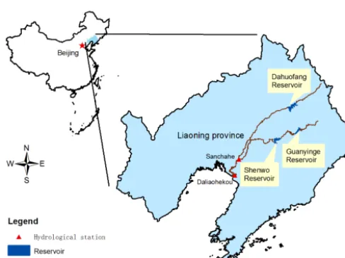
As shown in Fig. 3, the Dahuofang, Guanyinge, and Shenwo reservoirs compose the inter-basin multi-reservoir system in Liaoning province, China.
Liaoning province in China covers an area of 146×
ar-Table 2. Characteristics of each reservoir in the inter-basin multi-reservoir system.
Reservoir Active storage (106m3) Role in water
Flood season Non-flood season supply project
Dahuofang 1000 1430 Supplying water Guanyinge 1420 1420 Supplying water
and exporting water to Shenwo Shenwo 214 543 Supplying water
[image:6.612.164.436.85.204.2]and importing water from Guanyinge
Figure 3. Layout of the inter-basin multi-reservoir system.
eas, especially in the region between Daliaohekou and San-hekou hydrological stations.
The main purposes of the inter-basin multi-reservoir sys-tem are industrial water supply and agricultural water supply to eight cities (Shenyang, Fushun, Anshan, Liaoyang, Panjin, Yingkou, Benxi, and Dalian) of Liaoning province, and envi-ronmental water demands need to be satisfied fully. The char-acteristics of each reservoir in the inter-basin multi-reservoir system are illustrated in Table 2.
The flood season runs from July to September, during which the inflow takes up a large part of the annual in-flow. The active storage capacities of Dahuofang and Shenwo reservoirs reduce significantly during flood season for the flood control.
The inter-basin multi-reservoir operation system problem is formulated as follows: the objectives are minimization of industrial shortage index and minimization of agricultural shortage index as described in Eq. (1). With regard to the Shenwo reservoir, which has the same water supply oper-ation rule curve features as Dahuofang reservoir, the deci-sion variables include storage volumes on the industrial and agricultural curves and there are 39 decision variables.
Re-garding Guanyinge reservoir, the decision variables include storage volumes on the industrial curve and water transfer-ring curve due to the requirement of exporting water from Guanyinge reservoir to Shenwo reservoir in the inter-basin multi-reservoir system, which is similar to the water supply operation rule curve for industrial water demand, and there are 48 decision variables. Therefore, the inter-basin multi-reservoir system has six rule curves and 39×2+48=126 decision variables in total.
5 Results and discussions 5.1 Dahuofang reservoir
In the Dahuofang reservoir case study, a set of 2000 Latin hy-percube samples were used per decision variable yielding a total number of 2000×(39+2)=82 000 model simulations used to compute Sobol’s indices. Following the recommen-dations of Tang et al. (2007a, b) boot strapping the Sobol indices showed that 2000 samples per decision variable were sufficient to attain stable rankings of global sensitivity.
[image:6.612.45.289.228.411.2]Figure 4. First-order and total-order indices for the Dahuofang ROS
problem regarding (a) industrial shortage index and (b) agricultural shortage index. Thexaxis labels represent decision variables (water storage volumes on the industrial and agricultural curves).
sensitive variables in water supply operation rule curves for industrial and agricultural water demands will be provided in Sect. 5.1.3.
5.1.1 Simplified problems
Building on the sensitivity results shown in Fig. 4, one sim-plified version of the Dahuofang ROS problem is formulated: only 11 periods are considered for optimization, i.e., time pe-riods ind1, ind2, ind3, ind10, ind11, and ind12 for industrial curve and agr4-2, agr4-3, agr5-1, agr5-2, and agr5-3 for agri-cultural curve based on a total-order Sobol’s index thresh-old of greater than 10 %. The threshthresh-old is subjective and its ease-of-satisfaction decreases with increasing number of pa-rameters or parameter interactions. In all of the results for the Sobol’s method, parameters classified as the most sensi-tive contribute, on average, at least 10 percent of the overall model variance (Tang et al., 2007a, b). The full-search 39-period problem serves as the performance baseline relative to the reduced complexity problem.
5.1.2 Pre-conditioned optimization
In this section, the pre-conditioning methodology is demon-strated using the 11-period simplification of the Dahuofang ROS test case from the prior section, while the insensitive decision variables are set randomly first with domain knowl-edge and kept constant during the solution of the simplified problem.
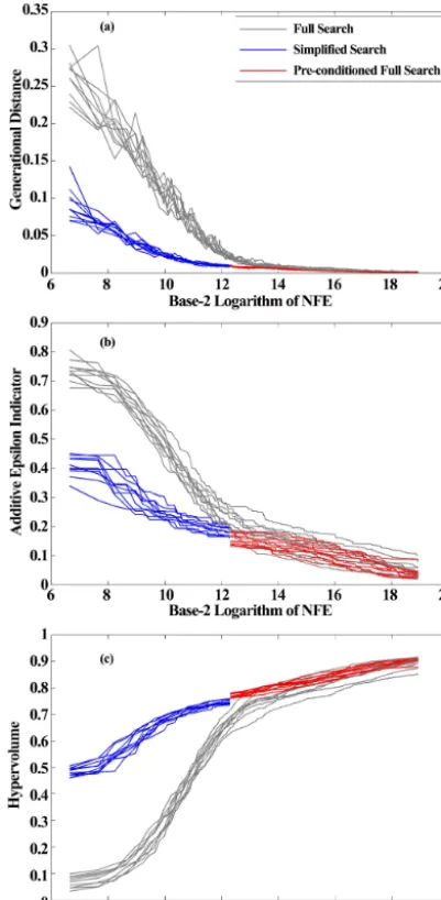
Using the sensitivity-informed methodology, the 11-period case was first solved usingε-NSGAII with a maxi-mum NFEs of 2000, and the Pareto-optimal solutions com-bined with the constant insensitive decision variables were then used as starting points to start a complete new search with a maximum NFEs of 498 000. The standard search us-ingε-NSGAII was set to a maximum NFEs of 500 000, so that the two methods have the same NFEs used for search. In this case, 10 random seed trials were used given the comput-ing resources available. The search traces in Fig. 5 show for all three metrics (generational distance, additive epsilon in-dicator, and hypervolume) that the complexity-reduced case can reliably approximate their portions of the industrial and agricultural water shortage trade-off given their dramatically reduced search periods. All three metrics show diminishing values at the end of the reduced search periods. The pre-conditioning results are shown in Fig. 5 in red search traces continuing from the blue reduced complexity search results.
Figure 5 clearly highlights that the sensitivity-informed pre-condition problems dramatically enhance search effi-ciency in terms of the generational distance, additive epsilon indicator, and hypervolume metrics. Overall, sensitivity-informed dimension reduction and pre-conditioning yield strong efficiency gains and a more reliable search (i.e., nar-rower band widths on search traces) for the Dahuofang ROS test case.
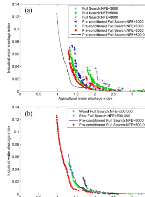
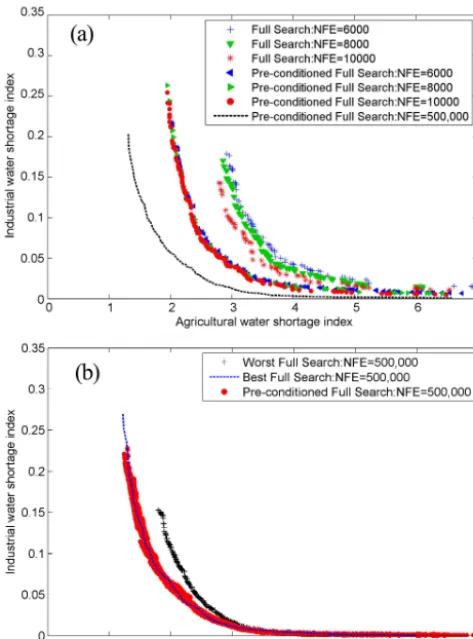
Figure 6a shows Pareto fronts from a NFEs of 3000, 5000, and 8000 in the evolution process of one random seed trial. In the case of the pre-conditioned search, the solutions from 3000, 5000, and 8000 evaluations are much better than the corresponding solutions in the case of standard baseline search. The results show that the Pareto-approximate front of the pre-conditioned search is much wider than that of the standard search, and clearly dominates that of the standard search in all the regions across the entire-objective space.
Figure 5. Performance metrics for the Dahuofang ROS problem
– (a) generational distance, (b) additive epsilon indicator, and (c) hypervolume.
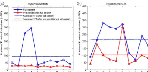
[image:8.612.308.546.64.388.2]Figure 7 shows the computational savings for two thresh-olds of hypervolume values 0.80 and 0.85 in the evolution process of each seed trial. In both cases of the thresholds of hypervolume values 0.80 and 0.85, NFEs of the pre-conditioned search is less than standard baseline search for each seed. In the case of the threshold of hypervolume value 0.80, the average NFEs of full search and pre-conditioned full search are approximately 94 564 and 25 083 for one seed run, respectively, and the computation is saved by 73.48 %. Although the NFEs of Sobol’s analysis are 82 000, the av-erage NFEs of pre-conditioned full search is approximately 25 083+82 000/10=33 283 for each seed run, and the computational saving is 64.80 %.
Figure 6. Pareto fronts derived from pre-conditioned and standard
full searches for the Dahuofang ROS problem. (a) Sample Pareto fronts with different numbers of function evaluations for one ran-dom seed trial. (b) The best and worst Pareto fronts of 10 seed trials.
Similarly, in the case of the threshold of hypervolume value 0.85, which is extremely difficult to achieve, the av-erage NFEs of full search and pre-conditioned full search are approximately 214 049 and 105 060 for each seed run, re-spectively, and the computation is saved by 50.92 %. When the computation demand by Sobol’s analysis is considered, the computational saving is still 47.09 %.
5.1.3 Optimal operation rule curves
The rule curves for Dahuofang reservoir from the final Pareto fronts based on the projected water demands and long-term historical inflow are shown in Fig. 8 (S2). The effectiveness and reasonability of the rule curves for Dahuofang reservoir are analyzed as follows.
Dur-Figure 7. Computational savings for two hypervolume values – (a) hypervolume=0.80 and (b) hypervolume=0.85.
ing the flood season, the curves also stay in low positions owing to the massive reservoir inflow and the requirement of flood control, so that it is beneficial to supply as much water as possible. However, during the season from mid-September to March, the curves remain high, especially from mid-September to October, in order to increase the proba-bility of limiting water supply and retaining enough water for later periods to avoid severe water supply shortages as drought occurs.
Second, Fig. 8 (S2) shows that different water demands oc-cur at different periods; e.g., industrial water demand ococ-curs throughout the whole year, and agricultural water demand occurs only at the periods from the second 10 days of April to the first 10 days of September. Especially during the flood season, there are still agricultural water demands due to tem-poral and spatial variations of rainfall though they are sig-nificantly reduced. Furthermore, note that the water supply curves are developed based on a historical, long-term rainfall series and the projected demands are also based on historical demands, covering stochastic uncertainties in demands and rainfalls. Due to the higher priority of industrial water ply than agricultural water supply, the industrial water sup-ply curve is closer to minimum storage throughout the year than the agricultural water supply curve. Due to the conflict-ing relationship between industrial and agricultural water de-mands, the industrial water supply curve is higher during the non-flood season, compared to the same curve in the flooding season. Thus, if the industrial water supply curve is too low during the non-flood season from January to April, which im-plies that the industrial water demand is satisfied sufficiently, there would not be enough water supplied for the agricul-tural water demand in the same year. Similarly, if the indus-trial water supply curve is too low during the non-flood sea-son from September to December, there would not be enough water supplied for the agricultural water demand in the next 1 or more years.
Third, the inflow and industrial water demands are rela-tively stable during the non-flood seasons from January to March and from October to December, so 1 month is taken as the scheduling time step, which is in accordance with the
re-Figure 8. Optimal rule curves for different solutions: (S0)
industry-favouring solution, (S1) agriculture-industry-favouring solution, and (S2) compromised solution.
quirement of Dahuofang reservoir operation in practice. Due to the larger amount of industrial water demand in periods 1, 2, 3, 10, 11, and 12 (January–March and October–December) than other periods, the water storages at these time periods are very important to industrial water supply, making them the most sensitive variables. Because the agricultural water demand is very high during the non-flood period from April to May, the agricultural water supply curve at this time period is higher, and the water storages at time periods from agr4-2 to agr5-3, i.e., the water storages at the first five time periods of the water supply operation rule curve for agricultural wa-ter demand, are the most important variables. On the other hand, in practice, if the agricultural water demand could not be satisfied at the first few periods of the water supply oper-ation rule curve, the agricultural water supply at each period throughout the year would be limited, i.e., the interactive ef-fects from variables are noticeable at time periods from agr4-2 to agr5-3.
Additionally, comparisons are made among the optimized solutions from the final Pareto fronts, including the industry-favouring solution (S0), agriculture-industry-favouring solution (S1), and compromised solution (S2). The comparisons of water shortage indices among different solutions are shown in Ta-ble 3, and the optimal rule curves for different solutions are shown in Fig. 8.
[image:9.612.49.289.66.182.2] [image:9.612.304.549.67.186.2]Table 3. Comparisons of water shortage indices among different solutions.
Solutions Water shortage index (–/no units)
Industrial Agricultural water demand water demand
(S0) Industry-favouring solution 0.000 3.550 (S1) Agriculture-favouring solution 0.020 1.380 (S2) Compromised solution 0.007 1.932
water supply curve; industrial and agricultural water short-age indices are 0.000 and 3.550, respectively. Opposite to S0, the agricultural water demand in S1 could be satisfied largely through lowering the agricultural water supply curve on the period from April to May and raising the industrial water supply curve; and industrial and agricultural water shortage indices are 0.020 and 1.380, respectively. Compared with so-lutions S0 and S1, two objectives are balanced in the compro-mised solution (S2), where industrial and agricultural water shortage indices are 0.007 and 1.932, respectively.
5.2 Inter-basin multi-reservoir system
5.2.1 Sensitivity analysis
Similarly to the Dahuofang case study, a set of 2000 Latin hypercube samples were used per decision variable yielding a total number of 2000×(126+2)=256 000 model simula-tions to compute Sobol’s indices in this case study.
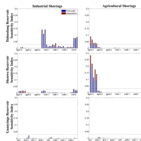
The first-order and total-order indices for 126 decision variables are shown in Fig. 9. Similarly to the results obtained from the Dahuofang ROS problem in Fig. 4, the variance in the two objectives, i.e., industrial and agricultural shortage indices, are largely controlled by the water storages at time periods from agr4-2 to agr5-3 of Shenwo reservoir water sup-ply operation rule curves for agricultural water demand, and the water storages at time periods from agr4-2 to agr5-3 of Dahuofang reservoir water supply operation rule curves for agricultural water demand, the water storages at time pe-riods ind1, ind2, ind3, ind7-1, ind10, ind11, and ind12 of Dahuofang reservoir water supply operation rule curves for industrial water demand based on a total-order Sobol’s in-dex threshold of greater than 3 %, which is subjective and its ease-of-satisfaction decreases with increasing numbers of pa-rameters or parameter interactions. These 17 time periods are obvious candidates for reducing the dimension of the origi-nal optimization problem and formulating a pre-conditioning problem. Therefore, the simplified problem is defined from the original design problem with the 109 intensive time pe-riods removed, while the insensitive decision variables are set randomly first with domain knowledge and kept constant during the solution of the simplified problem. The increased interactions across sensitive time periods in this test case
Figure 9. First-order and total-order indices for the inter-basin
multi-reservoir operation problem regarding industrial shortage in-dex and agricultural shortage inin-dex. Thexaxis labels represent de-cision variables (water storage volumes on the industrial, agricul-tural and water transferring curves).
should be noted; these interactions verify that this problem represents a far more challenging search problem.
5.2.2 Pre-conditioned optimization
[image:10.612.306.549.193.435.2]dis-Figure 10. Performance metrics for the inter-basin multi-reservoir
water supply operation problem – (a) generation distance, (b) addi-tive epsilon indicator, and (c) hypervolume.
tance, additive epsilon indicator, and hypervolume) that rep-resent performance metrics for the inter-basin multi-reservoir water supply operation system problem. Similarly, the pre-conditioning results are shown in Fig. 10 in red search traces continuing from the blue reduced complexity search results. It is clear that the sensitivity-informed pre-condition prob-lems enhance search efficiency in terms of the generational distance, additive epsilon indicator, and hypervolume met-rics. However, with the increase in problem complexity in comparison to the first case study (i.e., the number of deci-sion variables from 39 to 126), the search of the ROS opti-mization problem becomes more difficult, and so the met-rics obtained from the pre-conditioned search are not im-proved greatly compared with the standard baseline search.
Both Figs. 5 and 10 show that sensitivity-informed dimen-sion reduction and pre-conditioning could also yield strong efficiency gains and more reliable search (i.e., narrower band widths on search traces) for the inter-basin multi-reservoir system.
Figure 11a shows Pareto fronts from a NFEs of 6000, 8000 and 10 000 in the evolution process of one random seed trial. In the case of the pre-conditioned search, the so-lutions from the three NFE snapshots are much better than those from the standard baseline search. Similar to Fig. 6a, the results show that the Pareto-approximate front of the pre-conditioned search is much wider than that of the standard search, and clearly dominates that of the standard search in all the regions across the entire-objective space. Additionally, in the case of the pre-conditioned search, the solutions from 6000 evaluations are as good as those from 8000 evaluations and 10 000 evaluations. Furthermore, they are much better than the solutions from the standard baseline search. It should be noted that the slow progress in the Pareto-approximate fronts from 6000 to 10 000 evaluations reveals the difficulty of the inter-basin multi-reservoir operation system problem.
Figure 11b shows the best and worst Pareto fronts from a NFEs of 500 000 in the evolution process of 10 seed tri-als. Although it is obvious that the best Pareto-approximate front of the pre-conditioned is approximately as good as that of the standard search in all the regions across the entire-objective space, the Pareto solutions from 10 trials of the pre-conditioned search have significantly reduced variation, in-dicating a more reliable performance of the pre-conditioned method. In other words, the results show that the Pareto solu-tion from one random seed trial of the pre-condisolu-tioned search is as good as the best solution from 10 random seed trials of the standard search. That is to say, in the case of the pre-conditioned search, one random seed trial with a NFEs of 500 000 is sufficient to obtain the best set of Pareto solu-tions; however, in the case of the standard search, 10 seed trials with a total of 500 000×10=5 000 000 NFEs are re-quired to obtain the Pareto solutions. Note that the NFEs of Sobol’s analysis are 256 000, which is about half of the NFEs of one random seed trial. Thus, an improvement in search re-liability can significantly reduce the computational demand for a complex search problem such as the multi-reservoir case study, even when the computation required by sensitiv-ity analysis is included.
5.3 Discussions
[image:11.612.67.268.67.477.2]de-Figure 11. Pareto fronts derived from pre-conditioned and standard
full searches for the inter-basin multi-reservoir operation problem.
(a) Sample Pareto fronts with different numbers of function
evalua-tions for one random seed trial. (b) The best and worst Pareto fronts of 10 seed trials.
cision variables based on Sobol’s analysis. In the case of the inter-basin multi-reservoir operation system, the original op-timization problem has 126 decision variables, and the sim-plified problem has a significantly reduced number of de-cision variables, i.e., 17. Searching in such significantly re-duced space formed by sensitive decision variables makes it much easier to reach good solutions.
Although Sobol’s global sensitivity analysis is computa-tionally expensive, it captures the important sensitive infor-mation between a large number of variables for ROS models. This is critical for correctly screening insensitive decision variables and guiding the formulation of ROS optimization problems of reduced complexity (i.e., fewer decision vari-ables). For example, in the Dahuofang ROS problem, ac-counting for the sensitive information, i.e., using total-order or first-order indices, results in a simplified problem for a threshold of 10 % as shown in Fig. 4. Compared with the standard search, this sensitivity-informed method dramati-cally reduces the computational demands required for at-taining high-quality approximations of optimal ROS
trade-offs relationships between conflicting objectives, i.e., the best Pareto fronts from a NFEs of 8000 in the case of the pre-condition search are approximately the same as the best Pareto front from a NFEs of 500 000 in the case of the stan-dard baseline search.
In reality, for a very large and computationally intensive problem, the full search with all the decision variables would likely be so difficult that it may not be optimized sufficiently. However, as shown here, these simplified problems can be used to generate high-quality pre-conditioning solutions and thus dramatically improve the computational tractability of complex problems. The framework could be used for solving the complex optimization problems with a large number of decision variables.
For example, Fu et al. (2012) has used the framework for reducing the complexity of the multi-objective optimization problems in water distribution system (WDS), and applied it to two case studies with different levels of complexity – the New York tunnels rehabilitation problem and the Any-town water distribution network rehabilitation/redesign prob-lem. For the New York tunnels network, because the original optimization problem has 21 decision variables (pipes) and each variable has 16 options, the decision space is 1621=
1.934×1025. The simplified problem with eight decision variables based on Sobol’s analysis have a decision space of 168=4.295×10⁹. To obtain the same threshold of hyper-volume value 0.78 for the New York tunnels rehabilitation problem, the most pre-conditioned search need is 30 to 40 % of the NFEs compared to the full search through 50 random seed trials. In the case of the Anytown network, the origi-nal problem has a space of 2.859×1073, and the simplified problem has a significantly reduced space of 8.364×1038. Through 50 random seed trials for the Anytown rehabilita-tion/redesign problem, the full search requires an average of 800 000 evaluations to reach hypervolume value 0.77, and the pre-conditioned search exceeds the hypervolume value of 0.8 in all trials in fewer than 200 000 evaluations. The re-sults also show that searching in such significantly reduced space formed by sensitive decision variables makes it much easier to reach good solutions, and the sensitivity-informed reduction of problem size and pre-conditioning improve the efficiency, reliability, and effectiveness of the multi-objective evolutionary optimization.
[image:12.612.50.287.66.386.2]6 Conclusions
This study investigates the effectiveness of a sensitivity-informed optimization method for the ROS multi-objective optimization problems. The method uses a global sensitiv-ity analysis method to screen out insensitive decision vari-ables and thus forms simplified problems with a signifi-cantly reduced number of decision variables. The simplified problems dramatically reduce the computational demands re-quired to attain Pareto-approximate solutions, which them-selves can then be used to pre-condition and solve the orig-inal (i.e., full) optimization problem. This methodology has been tested on two case studies with different levels of com-plexity – the Dahuofang reservoir and the inter-basin multi-reservoir system in Liaoning province, China. The results ob-tained demonstrate the following:
1. The sensitivity-informed dimension reduction dramat-ically increases both the computational efficiency and effectiveness of the optimization process when com-pared to the conventional, full search approach. This is demonstrated in both case studies for both MOEA ef-ficiency (i.e., the NFEs required to attain high-quality trade-offs) and effectiveness (i.e., the quality approx-imations of optimal ROS trade-offs relationships be-tween conflicting design objectives).
2. The Sobol’s method can be used to successfully identify important sensitive information between different deci-sion variables in the ROS optimization problem and it is important to account for interactions between variables when formulating simplified problems.
Overall, this study illustrates the efficiency and effec-tiveness of the sensitivity-informed method and the use of global sensitivity analysis to inform dimension reduction. This method can be used for solving the complex multi-objective optimization problems with a large number of de-cision variables, such as optimal design of water distribution and urban drainage systems, distributed hydrological model calibration, multi-reservoir optimal operation and many other engineering optimization problems.
Acknowledgements. This study was supported by the China Postdoctoral Science Foundation grants (2014M561231), and Na-tional Natural Science Foundation of China grants (51320105010, 51279021, and 51409043).
Edited by: D. Solomatine
References
Castelletti, A., Pianosi, F., Quach, X., and Soncini-Sessa, R.: Assessing water reservoirs management and development in Northern Vietnam, Hydro l. Earth Syst. Sci., 16, 189–199, doi:10.5194/hess-16-189-2012, 2012.
Celeste, A. B. and Billib, M.: Evaluation of stochastic reservoir operation optimization models, Adv. Water Resour., 32, 1429– 1443, 2009.
Chang, F. J., Chen, L., and Chang, L. C.: Optimizing the reservoir operating rule curves by genetic algorithms, Hydrol. Process., 19, 2277–2289, 2005.
Chang, J. X., Bai, T., Huang, Q., and Yang, D. W.: Optimization of water resources utilization by PSO-GA, Water Resour. Manag., 27, 3525–3540, 2013.
Chen, L.: Real coded genetic algorithm optimization of long term reservoir operation, J. Am. Water Resour. As., 39, 1157–1165, 2003.
Draper, A. J. and Lund, J. R.: Optimal hedging and carryover stor-age value, J. Water Res. Pl.-ASCE, 130, 83–87, 2004.
François, B., Hingray, B., Hendrickx, F., and Creutin, J. D.: Sea-sonal patterns of water storage as signatures of the climatological equilibrium between resource and demand, Hydrol. Earth Syst. Sci., 18, 3787–3800, doi:10.5194/hess-18-3787-2014, 2014. Fu, G. T., Kapelan, Z., and Reed, P.: Reducing the complexity of
multi-objective water distribution system optimization through global sensitivity analysis, J. Water Res. Pl.-ASCE, 138, 196– 207, 2012.
Goor, Q., Halleux, C., Mohamed, Y., and Tilmant, A.: Optimal operation of a multipurpose multireservoir system in the East-ern Nile River Basin, Hydrol. Earth Syst. Sci., 14, 1895–1908, doi:10.5194/hess-14-1895-2010, 2010.
Huang, W. C., Harboe, R., and Bogardi, J. J.: Testing stochastic dynamic programming models conditioned on observed or fore-casted inflows, J. Water Res. Pl.-ASCE 117, 28–36, 1991. Karamouz, M. and Houck, M. H.: Annual and monthly reservoir
operating rules generated by deterministic optimization, Water Resour. Res., 18, 1337–1344, 1982.
Ko, S. K., Oh, M. H., and Fontane, D. G.: Multiobjective analysis of service-water-transmission systems, J. Water Res. Pl.-ASCE, 132, 78–83, 1997.
Kollat, J. B. and Reed, P. M.: Comparing state-of-the-art evolution-ary multi-objective algorithms for long-term groundwater moni-toring design, Adv. Water Resour., 29, 792–807, 2006.
Kollat, J. B. and Reed, P. M.: A computational scaling analysis of multiobjective evolutionary algorithms in long-term groundwater monitoring applications, Adv. Water Resour., 30, 408–419, 2007. Koutsoyiannis, D. and Economou, A.: Evaluation of the parameterization- simulation-optimization approach for the con-trol of reservoir systems, Water Resour. Res., 39, WES2.1– WES2.17, 2003.
Labadie, J. W.: Optimal operation of multireservoir systems: state-of-the-art review, J. Water Res. Pl.-ASCE, 130, 93–111, 2004. Liu, P., Guo, S. L., Xu, X. W., and Chen, J. H.: Derivation of
aggregation-based joint operating rule curves for cascade hy-dropower reservoirs, Water Resour. Manag., 25, 3177–3200, 2011a.
Momtahen, S. and Dariane, A. B. Direct search approaches using genetic algorithms for optimization of water reservoir operating policies, J. Water Res. Pl.-ASCE, 133, 202–209, 2007.
Mousavi, H. and Ramamurthy, A. S.: Optimal design of multi-reservoir systems for water supply, Adv. Water Resour., 23, 613– 624, 2000.
MWR-PRC (Ministry of Water Resources of PRC): China Wa-ter Resources Bulletin, China WaWa-ter Resources and Hydropower Press, Beijing, China, 2008 (in Chinese).
Nalbantis, I. and Koutsoyiannis, D.: A parametric rule for planning and management of multiple-reservoir systems, Water Resour. Res., 33, 2165–2177, 1997.
Nicklow, J., Reed, P. M., Savic, D., Dessalegne, T., Harrell, L., Chan-Hilton, A., Karamouz, M., Minsker, B., Ostfeld, A., Singh, A., and Zechman, E.: State of the art for genetic algorithms and beyond in water resources planning and management, J. Water Res. Pl.-ASCE, 136, 412–432, 2010.
Oliveira, R. and Loucks, D. P.: Operating rules for multireservoir systems, Water Resour. Res., 33, 839–852, 1997.
Powell, W. B.: Approximate Dynamic Programming: Solving the Curses of Dimensionality, John Wiley & Sons Inc., New York City, USA, ISBN-13: 9780470171554, 2007.
Sadegh, M., Mahjouri, H., and Kerachian, R.: Optimal inter-basin water allocation using crisp and fuzzy shapely games, Water Re-sour. Manag., 24, 2291–2310, 2010.
Shiau, J.-T.: Analytical optimal hedging with explicit incorporation of reservoir release and carryover storage targets, Water Resour. Res., 47, W01515, doi:10.1029/2010WR009166, 2011. Shiau, J.-T. and Lee, H.-C.: Derivation of optimal hedging rules for
a water-supply reservoir through compromise programming, Wa-ter Resour. Manag., 19, 111–132, 2005.
Shih, J. S. and ReVelle, C.: Water supply operations during drought: a discrete hedging rule, Eur. J. Oper. Res., 82, 163–175, 1995. Shirangi, E., Kerachian, R., and Bajestan, M. S.: A simplified model
for reservoir operation considering the water quality issues: Ap-plication of the Young conflict resolution theory, Environ. Monit. Assess., 146, 77–89, 2008.
Simonovic, S. P.: Reservoir systems analysis: closing gap between theory and practice, J. Water Res. Pl.-ASCE, 118, 262–280, 1992.
Srinivasan, K. and Philipose, M. C.: Effect of hedging on over-year reservoir performance, Water Resour. Manag., 12, 95–120, 1998. Suen, J. P. and Eheart, J. W.: Reservoir management to balance ecosystem and human needs: Incorporating the paradigm of the ecological flow regime, Water Resour. Res., 42, W03417, doi:10.1029/2005WR004314, 2006.
Tang, Y., Reed, P., and Wagener, T.: How effective and effi-cient are multiobjective evolutionary algorithms at hydrologic model calibration?, Hydrol. Earth Syst. Sci., 10, 289–307, doi:10.5194/hess-10-289-2006, 2006.
Tang, Y., Reed, P. M., van Werkhoven, K., and Wagener, T.: Ad-vancing the identification and evaluation of distributed rainfall-runoff models using global sensitivity analysis, Water Resour. Res., 43, W06415, doi:10.1029/2006WR005813, 2007a.
Tang, Y., Reed, P., Wagener, T., and van Werkhoven, K.: Comparing sensitivity analysis methods to advance lumped watershed model identification and evaluation, Hydrol. Earth Syst. Sci., 11, 793– 817, doi:10.5194/hess-11-793-2007, 2007b.
Teegavarapu, R. S. V. and Simonovic, S. P.: Optimal operation of water resource systems: trade-offs between modeling and practi-cal solutions, in: Integrated water resources management, edited by: Mariño, M. A. and Simonovic, S. P., 272, IAHS Publ., Wallingford, UK, 257–263, 2001.
Tejada-Guibert, J. A., Johnson, S. A., and Stedinger, J. R.: The value of hydrologic information in stochastic dynamic programming models of a multireservoir system, Water Resour. Res., 31, 2571– 2579, 1995.
Tu, M.-Y., Hsu, N.-S., and Yeh, W. W.-G.: Optimization of reservoir management and operation with hedging rules, J. Water Res. Pl.-ASCE, 129, 86–97, 2003.
Tu, M.-Y., Hsu, N.-S., Tsai, F. T.-C., and Yeh, W. W.-G.: Optimiza-tion of hedging rules for reservoir operaOptimiza-tions, J. Water Res. Pl.-ASCE, 134, 3–13, 2008.
Veldhuizen, D. A. V. and Lamont, G. B.: Evolutionary Computa-tion and Convergence to a Pareto Front, in: Late Breaking Papers at the Genetic Programming Conference, edited by: Koza, J. R., Stanford University Bookstore, Madison, Wisconsin, US, 221– 228, 1998.
Wurbs, R. A.: Reservoir-system simulation and optimization mod-els, J. Water Res. Pl.-ASCE, 119, 455–472, 1993.
Xu, W., Zhang, C., Peng, Y., Fu, G. T., and Zhou, H. C.: A two stage Bayesian stochastic optimisation model for cascaded hydropower systems considering varying uncer-tainty of flow forecasts, Water Resour. Res., 50, 9267–9286, doi:10.1002/2013WR015181, 2014.
Yeh, W. W.-G.: Reservoir management and operations models: a state-of-the-art review, Water Resour. Res., 21, 1797–1818, 1985.
Young, G. K.: Finding, reservoir operating rules, Journal of Hy-draulic Division, 93, 297–321, 1967.
Zhang, C., Chu, J. G., and Fu, G. T.: Sobol’s sensitivity analysis for a distributed hydrological model of Yichun River Basin, China, J. Hydrol., 480, 58–68, 2013.
Zhang, H. F., Zhou, J. Z., Fang, N., Zhang, R., and Zhang, Y. C.: An efficient multi-objective adaptive differential evolution with chaotic neuron network and its application on long-term hydropower operation with considering ecological environment problem, Electrical Power and Energy Systems, 45, 60–70, 2013. Zhao, T. T. G., Zhao, J. S., and Yang, D. W.: Improved dynamic programming for hydropower reservoir operation, J. Water Res. Pl.-ASCE, 140, 365–374, 2014.
Zitzler, E. and Thiele, L.: Multiobjective optimization using evo-lutionary algorithms-a comparative case study, in: Parallel prob-lem solving from nature (PPSN V), Lecture notes in computer science, edited by: Eiben, A., Back, T., Schoenauer, M., and Schwefel, H.-P., Springer-Verlag, Berlin, Germany, Amsterdam, the Netherlands, 292–301, 1998.