Development of a large sample watershed scale hydrometeorological data set for the contiguous USA: data set characteristics and assessment of regional variability in hydrologic model performance

www.hydrol-earth-syst-sci.net/19/209/2015/ doi:10.5194/hess-19-209-2015

© Author(s) 2015. CC Attribution 3.0 License.

Development of a large-sample watershed-scale hydrometeorological

data set for the contiguous USA: data set characteristics and

assessment of regional variability in hydrologic model performance

A. J. Newman1, M. P. Clark1, K. Sampson1, A. Wood1, L. E. Hay2, A. Bock2, R. J. Viger2, D. Blodgett3, L. Brekke4, J. R. Arnold5, T. Hopson1, and Q. Duan6

1_{National Center for Atmospheric Research, Boulder CO, USA}

2_{United States Geological Survey, Modeling of Watershed Systems, Lakewood CO, USA} 3_{United States Geological Survey, Center for Integrated Data Analytics, Middleton WI, USA} 4_{US Department of Interior, Bureau of Reclamation, Denver CO, USA}

5_{US Army Corps of Engineers, Institute for Water Resources, Seattle WA, USA} 6_{Beijing Normal University, Beijing, China}

Correspondence to: A. J. Newman ([email protected])

Received: 17 April 2014 – Published in Hydrol. Earth Syst. Sci. Discuss.: 28 May 2014 Revised: 23 November 2014 – Accepted: 1 December 2014 – Published: 14 January 2015

Abstract. We present a community data set of daily forc-ing and hydrologic response data for 671 small- to medium-sized basins across the contiguous United States (median basin size of 336 km2) that spans a very wide range of hy-droclimatic conditions. Area-averaged forcing data for the period 1980–2010 was generated for three basin spatial con-figurations – basin mean, hydrologic response units (HRUs) and elevation bands – by mapping daily, gridded meteoro-logical data sets to the subbasin (Daymet) and basin poly-gons (Daymet, Maurer and NLDAS). Daily streamflow data was compiled from the United States Geological Survey Na-tional Water Information System. The focus of this paper is to (1) present the data set for community use and (2) provide a model performance benchmark using the coupled Snow-17 snow model and the Sacramento Soil Moisture Account-ing Model, calibrated usAccount-ing the shuffled complex evolution global optimization routine. After optimization minimizing daily root mean squared error, 90 % of the basins have Nash– Sutcliffe efficiency scores ≥0.55 for the calibration period and 34 %≥0.8. This benchmark provides a reference level of hydrologic model performance for a commonly used model and calibration system, and highlights some regional varia-tions in model performance. For example, basins with a more pronounced seasonal cycle generally have a negative low flow bias, while basins with a smaller seasonal cycle have a

positive low flow bias. Finally, we find that data points with extreme error (defined as individual days with a high fraction of total error) are more common in arid basins with limited snow and, for a given aridity, fewer extreme error days are present as the basin snow water equivalent increases.

1 Introduction

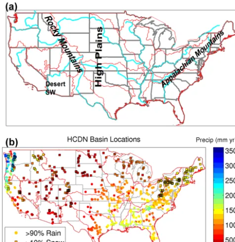
Figure 1. (a) Contiguous United States (CONUS) with states (gray), rivers (blue) and major hydrologic regions (red). Text in-dicates major geographic regions discussed in text. (b) Location of the 671 HCDN-2009 basins across the contiguous US used in the basin data set with precipitation shaded. Circles denote basins with>90 % of their precipitation falling as rain, squares with black outlines denote basins with>10 % of their precipitation falling as snow as determined by using a 0◦C daily mean Daymet tempera-ture threshold. State outlines are in thin gray and hydrologic regions in thin red.

The Model Parameter Estimation Project (MOPEX) data set does provide basin mean hydrometeorological data and ob-served streamflow records for 438 basins across the contigu-ous United States (CONUS; Schaake et al., 2006) for over more than 30 years; making it one of the few, high-quality, freely available hydrometeorological data sets with immedi-ate applicability to catchment-type hydrologic models.

Gupta et al. (2014) emphasize that more large-sample hy-drologic studies are needed to “balance depth with breadth”; most hydrologic studies have traditionally focused on one or a small number of basins (depth), which hinders the ability to establish general hydrologic concepts applicable across re-gions (breadth). Gupta et al. (2014) go on to discuss practi-cal considerations for large-sample hydrology studies, noting first and foremost that large data sets of quality basin data need to be available and shared in the community. In support of this philosophy, we present a large-sample hydrometeo-rological data set and modeling tools to understand regional variability in hydrologic model performance across the con-tiguous US (Fig. 1). The development of the basin data set presented herein takes advantage of high-quality, freely available data from various US government agencies and

re-search laboratories. It includes (1) daily forcing data for 671 basins for multiple spatial configurations over the 1980–2010 time period; (2) daily streamflow data; (3) basic metadata (e.g., location, elevation, size, and basin delineation shape-files) and (4) benchmark model performance which contains the final calibrated model parameter sets, model output time series for all basins as well as summary graphics for each basin. This builds on the MOPEX data set by providing basin mean forcing data for 233 more basins along with two other spatial configurations and the benchmark model performance parameter sets and model output.

This data set and benchmark application is intended for the community to use as a test bed to facilitate the evalu-ation of hydrologic modeling and prediction questions. To this end, the benchmark consists of the calibrated, coupled Snow-17 snow model and the Sacramento Soil Moisture Ac-counting Model (SAC-SMA) for all 671 basins using the shuffled complex evolution (SCE) global optimization rou-tine. Development of a large-sample hydrologic data set such as this will allow for exploration into many important scien-tific questions. We provide some basic analysis relating to questions such as (1) what is the model performance across a large sample of basins and how does model performance vary across basin hydroclimatic conditions? (2) How do er-ror characteristics relate to basin calibration performance and hydroclimatic conditions? This basic analysis is intended to highlight some of the important questions that can be an-swered through large-sample hydrologic studies and provide example results for further exploration.

The next section describes the development of the basin data set from basin selection through forcing data genera-tion. It then briefly describes the modeling system and cal-ibration routine. Next, example results using the basin data set and modeling platform are presented. Finally, concluding thoughts and next steps are discussed.

2 Basin data set

The development of a freely available large-sample basin data set requires several choices and subsequent data acqui-sition. Three major decisions were made and are discussed in this section: (1) the selection process for the basins, (2) the various basin spatial configurations to be developed, and (3) selection of the underlying forcing data set used to de-velop forcing data time series. Additionally, aggregation of the necessary streamflow data is described.

2.1 Basin selection

USGS. As a subset of the GAGES-II database, a portion of the basins with minimal human disturbance (i.e., mini-mal land use changes or disturbances, minimini-mal human wa-ter withdrawals) are noted as “reference” gages. A further subsetting of the reference gages were made as a follow-on to the Hydro-Climatic Data Network (HCDN) 1988 data set (Slack and Landwehr, 1992). These gages, marked HCDN-2009 (Lins, 2012), meet the following criteria: (1) have at least 20 years of complete flow data between 1990 and 2009 and were active as of 2009, (2) are a GAGES-II reference gage, (c) have less than 5 % imperviousness as measured by the National Land Cover Database (NLCD-2011; Jin et al., 2013), and (d) passed a manual survey of human impacts in the basin by local Water Science Center evaluators (Falcone et al., 2010). There are 704 gages in the GAGES-II database that are considered HCDN-2009 across the CONUS. This study uses that portion of the HCDN-2009 basin set as the starting point since they should best represent natural flow conditions. After initial processing and data availability re-quirements, 671 basins are used for analysis in this study (Fig. 1b). Because these basins have minimal human in-fluence they are almost exclusively smaller, headwater-type basins.

2.2 Forcing and streamflow data

Hydrologic models are run with a variety of spatial con-figurations, including entire watersheds (lumped), elevation bands, hydrologic response units (HRUs), or grids. For this data set, forcing data were calculated (via areal averaging) for watershed, HRU and elevation band spatial configura-tions. The basin spatial configurations were created from the base national geospatial fabric for hydrologic modeling developed by the USGS Modeling of Watershed Systems (MoWS) group (Viger, 2014; Viger and Bock, 2014). The geospatial fabric is a watershed-oriented analysis of the Na-tional Hydrography Data set that contains points of interest (e.g., USGS streamflow gauges), hydrologic response unit boundaries and simplified stream segments (not used in this study). This geospatial fabric contains points of interest that include USGS streamflow gauges and allowed for the de-termination of upstream total basin area and basin HRUs (Viger, 2014; Viger and Bock, 2014). A digital elevation model (DEM) was applied to the geospatial fabric data set to create elevation contour polygon shapefiles for each basin. The USGS Geo Data Portal (GDP) developed by the USGS Center for Integrated Data Analytics (CIDA) (Blodgett et al., 2011) was leveraged to produce area-weighted forcing data for the various basin spatial configurations over our time pe-riod. The GDP performs all necessary spatial subsetting and weighting calculations and returns the area-weighted time se-ries for the specified inputs.

The Daymet data set was selected as the primary gridded meteorological data set to derive forcing data for our stream-flow simulations (Thornton et al., 2012). Daymet was

cho-sen because of its high spatial resolution, a necessary re-quirement to more fully estimate spatial heterogeneity for basins in complex topography. Daymet is a daily, gridded (1×1 km) data set over the CONUS and southern Canada and is available from 1980 to present. It is derived solely from daily observations of temperature and precipitation. The Daymet variables used here are daily maximum and min-imum temperature, precipitation, shortwave downward ra-diation, day length, and humidity; additionally, snow water equivalent is included (not used in this work). These daily values are estimated through the use of an iterative method dependent on local station density and the spatial convolution of a truncated Gaussian filter for station interpolation, and the Mountain Climate Simulator (MT-CLIM) to estimate short-wave radiation and humidity (Thornton et al., 1997; Thorn-ton and Running, 1999; ThornThorn-ton et al., 2000). Daymet does not include estimates of potential evapotranspiration (PET), a commonly needed input for conceptual hydrologic models or wind speed and direction. Therefore, PET was estimated using the Priestly–Taylor (P–T) method (Priestly and Tay-lor, 1972) and is discussed further in Sect. 3. Data quality is an ever-present issue in hydrologic modeling, and while the input data to Daymet are subject to rigorous quality control checks (Durre et al., 2008, 2010) potential errors may remain (Menne et al., 2009, 2010; Oubeidillah et al., 2013). Addi-tionally, the Maurer et al. (2002) and National Land Data As-similation System (NLDAS) (Xia et al., 2012) 12 km gridded data sets were processed to provide daily forcing data for the basin lumped configuration, resulting in three distinct data sets available for future forcing data impact studies.

Daily streamflow data for the HCDN-2009 gages were obtained from the USGS National Water Information Sys-tem server (http://waterdata.usgs.gov/usa/nwis/sw) over the same forcing data time period, 1980–2010. While the pe-riod 1980–1990 is not covered by the HCDN-2009 review, it was assumed that these basins would have minimal hu-man disturbances in this time period as well. For the portion of the basins that do not have streamflow records back to 1980, analysis is restricted to the available data records. The USGS provides streamflow data flags to identify periods of estimated flow and are included here. However, other data quality information is unavailable without further investiga-tion and not available in this data set. For reference, 90 % (604) of the basins have 20 % or fewer flow days estimated and 75 % (503 basins) have 10 % or less flow values esti-mated.

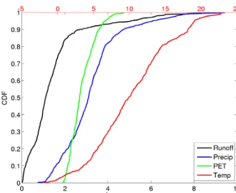
Figure 2. Annual CDFs of runoff (mm day−1) (black, bottomx

axis), precipitation (mm day−1) (blue, bottom x axis), potential evapotranspiration (mm day−1)(green, bottomxaxis), and temper-ature (◦C) (red, topxaxis).

Daymet-estimated basin mean temperatures range from −2 to 23◦C with precipitation amounts of 0.7–9.4 mm day−1 (Fig. 2). Annual observed mean runoff ranges from 0.01 to 9.3 mm day−1 with PET estimates ranging from 1.9 to 4.8 mm day−1. Interestingly, this implies that Daymet precip-itation itself is not enough to balance the observed runoff in some basins and is consistent with other recent large-sample hydrologic studies (Oubeidillah et al., 2013). Seasonal vari-ations in these four variables are large as well, with some basins reaching mean winter time temperatures lower than −10◦C and summer time mean temperatures higher than 25◦C (not shown). The seasonal water balance varies greatly with some basins experiencing much higher precipitation and runoff rates in one season versus another (e.g., spring runoff peaks in mountain snowmelt-dominated basins). As expected, PET varies seasonally with a minimum in winter and a maximum in summer.

Figure 3 gives CDFs for various physical descriptors of the basin set. The basins range in size from roughly 1 to 25 800 km2with the median basin size being about 335 km2 and have mean elevations spanning from nearly sea level (10 m) to high alpine elevations (3570 m) with a median el-evation of 462 m. Notably, 75 basins have mean elel-evations >2000 m. Corresponding to the large range of elevations in the basin set, the mean slopes vary considerably, span-ning over 2 orders of magnitude from near zero to over 200 m km−1. The basin set covers a wide range of basin shapes with aspect ratios ranging from 0.08 to about 11. Fi-nally, there is a large range of forest covers across the basin set which may have implications for hydrologic similarity (Oudin et al., 2010) with 20 % of the basins having less than

Figure 3. Cumulative density functions of basin size (km2)(black), basin mean elevation (m) (red), mean slope (m km−1)(blue), and fractional forest cover (green) for the basin set.

(more than) 14 % (98 %) forest cover and the median basin having about 80 % forest cover (NLCD-2011).

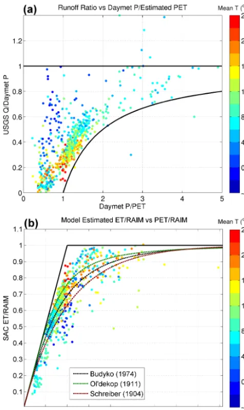
Figure 4. (a) Runoff ratio of observed runoff to Daymet-estimated precipitation versus ratio of Daymet-estimated precipitation to Priestly–Taylor-estimated PET. (b) Model-derived Budyko analy-sis using model ET, PET and total surface water input (rain plus melt, RAIM) for the 671 basins and three derivations of the Budyko curve (dashed lines). Basin mean temperature is shaded (coloring) in both panels.

in the forcing or streamflow data sets and permits any iden-tified errors to be placed into spatial and temporal context, a benefit of large-sample studies.

As noted above, no additional quality control was per-formed on the candidate basins before calibration. For com-pleteness and to more fully highlight some of the benefits and tradeoffs made when performing large-sample hydro-logic studies, all basins are kept for analysis in this work.

3 Hydrologic modeling benchmark

As stated in the introduction, the intended purpose of this data set is a test bed to facilitate assessment of hydrologic modeling and prediction questions across broad hydrocli-matic variations, and we focus here on providing a bench-mark performance assessment for a widely used calibrated, conceptual hydrologic modeling system. This type of data set can be used for many applications including evaluation of new modeling systems against a well known benchmark sys-tem over wide ranging conditions, or as a base for compre-hensive predictability experiments exploring the importance of meteorology or initial basin conditions. To this end, we have implemented and tested an initial model and calibration system described below, using the primary models and objec-tive calibration approach that have been used by the US Na-tional Weather Service River Forecast Centers (NWSRFCs) in service of operational short-term and seasonal streamflow forecasting.

3.1 Models

The HCDN-2009 basins include those with substantial sea-sonal snow cover (Fig. 1b), necessitating a snow model in ad-dition to a hydrologic model. Within the NWSRFCs, the cou-pled Snow-17 and SAC-SMA system is used. Snow-17 is a conceptual air-temperature-index-based snow accumulation and ablation model (Anderson, 1973). It uses near-surface air temperature to determine the energy exchange at the snow– air interface and the only time-varying inputs are typically air temperature and precipitation (Anderson, 1973, 2002). The SAC-SMA model is a conceptual hydrologic model that in-cludes representation of physical processes such as evapo-transpiration, percolation, surface flow, and subsurface lat-eral flow. Required inputs to SAC-SMA are potential evap-otranspiration and water input to the soil surface (Burnash et al., 1973; Burnash, 1995). Snow-17 runs first and deter-mines the partition of precipitation into rain and snow and the evolution of the snowpack. Any rain, snowmelt or rain pass-ing unfrozen through the snowpack for a given time step be-comes direct input to the SAC-SMA model. Finally, stream-flow routing is accomplished through the use of a simple two-parameter, Nash-type instantaneous unit-hydrograph model (Nash, 1957).

3.2 Calibration

soil moisture state that was allowed to spin down to equilib-rium for a given basin by running the first year of the calibra-tion period repeatedly and assumed no initial snowpack. This was done until all SAC-SMA state variables had minimal year over year variations, which is a spin-up approach used by the Project for Intercomparison of Land-Surface Process Schemes (e.g., Schlosser et al., 2000). Determination of opti-mal calibration sampling and spin-up procedures is an area of active research. Spin-up was performed for every parameter set specified by the optimization algorithm, then the model was integrated for the calibration period and the RMSE (root mean square error) for that parameter set was calculated.

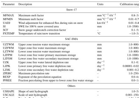
Objective calibration was done by minimizing the RMSE of daily modeled runoff versus observed streamflow us-ing the SCE global search algorithm of Duan et al. (1992, 1993). The SCE algorithm uses a combination of probabilis-tic and determinisprobabilis-tic optimization approaches that systemat-ically spans the allowed parameter search space and also in-cludes competitive evolution of the parameter sets (Duan et al., 1993). Prior applications to the SAC-SMA model have shown good results (Sorooshian et al., 1993; Duan et al., 1994). In the coupled Snow-17 and SAC-SMA modeling sys-tem, 35 potential parameters are available for calibration, of which we calibrated 20 parameters having either a priori es-timates (Koren et al., 2000) or those found to be most sen-sitive following Anderson (2002) (Table 1). The SCE algo-rithm was run using 10 different random seed starts for the initial parameter sets for each basin, in part to evaluate the robustness of the optimum in each case, and the optimized parameter set with the minimum RMSE from the 10 differ-ent optimization runs was chosen for evaluation.

For Snow-17, six parameters were chosen for optimiza-tion (Table 1): the minimum and maximum melt factors (MFMIN, MFMAX), the wind adjustment for enhanced en-ergy fluxes to the snowpack during rain on snow (UADJ), the rain/snow partition temperature, which may not be 0◦C (PXTEMP), the snow water equivalent for 100 % snow cov-ered area (SI), and the gauge catch correction term for snow-fall only (SCF). These six parameters were chosen because MFMIN, MFMAX, UADJ, SCF, and SI are defined as major model parameters by Anderson (2002). PXTEMP was also shown to be important in the Snow-17 model by Mizukami et al. (2013). The SCF is critical in many snow-dominated basins as precipitation is generally underestimated in these types of basins (e.g., Yang et al., 1998) and is certainly un-derestimated in some basins in Daymet as shown in Figs. 3 and 4.

The areal depletion curve (ADC) is considered a major parameter in Snow-17. However, to avoid expanding the parameter space by the number of ordinates on the curve (typically 10), we manually specified the ADC according to regional variations in latitude, topographic characteristics (e.g., plains, hills or mountains) and typical air mass char-acteristics (e.g., maritime polar, continental polar) (as sug-gested in Anderson, 2002). The remaining Snow-17

parame-ters were set in the same manner. Following the availability of a priori parameter estimates for SAC-SMA from a vari-ety of data sets and various calibration studies with SAC-SMA (Koren et al., 2000; Anderson et al., 2006; Pokhrel and Gupta, 2010; Zhang et al., 2012), 11 parameters from SAC-SMA are included for calibration (Table 1). We use an in-stantaneous unit hydrograph, represented as a two-parameter gamma distribution for streamflow routing (Sherman, 1932; Clark, 1945; Nash, 1957; Dooge, 1959), the parameters of which were inferred as part of calibration. .

Finally, the scaling parameter in the Priestly–Taylor PET estimate is also calibrated. The P–T equation (Priestly and Taylor, 1972) can be written as

PET=a λ·

s·(Rn−G)

s+γ . (1)

Where λ (MJ kg−1) is the latent heat of vaporization, Rn (MJ m−2day−1)is the net radiation estimated using day of year, all Daymet variables and equations to estimate the vari-ous radiation terms (Allen et al., 1988; Zotarelli et al., 2009), G(MJ m−2day−1)is the soil heat flux (assumed to be zero in this case),s(kPa◦C−1)is the slope of the saturation vapor pressure–temperature relationship,γ (kPa◦C−1)is the psy-chrometric constant anda (unitless) is the P–T coefficient. The P–T coefficient replaces the aerodynamic term in the Penman–Monteith equation and varies by the typical condi-tions of the area where the P–T equation is being applied with humid forested basins typically having smaller values and exposed arid basins having larger values (Shuttleworth and Calder, 1979; Morton, 1983; Jensen et al., 1990). Thus, the P–T coefficient was included in the calibration since it should vary from basin to basin.

4 Benchmark results

4.1 Assessment objectives and metrics

Table 1. Table describing all parameters calibrated and their bounds for calibration.

Parameter Description Units Calibration range

Snow-17

MFMAX Maximum melt factor mm◦C−16 h−1 0.8–3.0

MFMIN Minimum melt factor mm◦C−16 h−1 0.01–0.79

UADJ Wind adjustment for enhanced flux during rain on snow km 6 h−1 0.01–0.40

SI SWE for 100 % snow covered area mm 1.0–3500.0

SCF Snow gauge undercatch correction factor – 0.1–5.0

PXTEMP Temperature of rain/snow transition ◦C −1.0–3.0

SAC-SMA

UZTWM Upper zone tension water maximum storage mm 1.0–800.0

UZFWM Upper zone free water maximum storage mm 1.0–800.0

LZTWM Lower zone tension water maximum storage mm 1.0–800.0

LZFPM Lower zone free water primary maximum storage mm 1.0–1000.0

LZFSM Lower zone free water secondary maximum storage mm 1.0–1000.0

UZK Upper zone free water lateral depletion rate day−1 0.1–0.7

LZPK Lower zone primary free water depletion rate day−1 0.00001–0.025 LZSK Lower zone secondary free water depletion rate day−1 0.001–0.25

ZPERC Maximum percolation rate – 1.0–250.0

REXP Exponent of the percolation equation – 0.0–6.0

PFREE Fraction percolating from upper to lower zone free water storage – 0.0–1.0

Others

USHAPE Shape of unit hydrograph – 1.0–5.0

USCALE Scale of unit hydrograph – 0.001–150.0

P–T Priestly–Taylor coefficient – 1.26–1.74

the long-term monthly mean flow instead of mean flow (de-noted MNSE hereafter), thus preventing climatological sea-sonality from inflating the NSE and more accurately rank-ing basins by the degree to which the model added value over climatology in response to weather events (Garrick et al., 1978; Martinec and Rango, 1989; Schaefli et al., 2005). MNSE in this context is defined for each day of year (DOY) via a 31-day window centered on a given DOY. The long-term flow for that 31-day “month” is computed giving rise to a “monthly” mean flow. Using this type of climatology as the base for an NSE-type analysis provides improved standard-ization in basins with large flow autocorrelations. This defi-nition is similar to the one proposed by Garrick et al. (1978) but with the addition of the 31-day smoother, which is done to provide a smoother reference climatology.

Also, several other advanced, more physically based, met-rics of model performance are provided. First, three diag-nostic signatures based on the flow duration curve (FDC) from Yilmaz et al. (2008) are computed: (1) the top 2 % flow bias, (2) the bottom 30 % flow bias, and (3) the bias of the slope of the middle portion (20–70 percentile) of the FDC. Second, examination of the time series of squared error contribution to the RMSE statistic was performed to high-light events in which the model performs poorly following Clark et al. (2008). This analysis was performed to gauge

the representativeness of performance metrics over the model record by using the sorted (highest to lowest) time series of squared error to identify theN number of the largest error days and determine their fractional error contribution to the total. Finally, we extend this analysis to introduce a simple, normalized general error index for application and compari-son across varying modeling and calibration studies. We coin the index, E50, the fraction of calibration points contributing 50 % of the error. This captures the number of points deter-mining the majority of the error and thus the optimal param-eter set.

4.2 Spatial variability

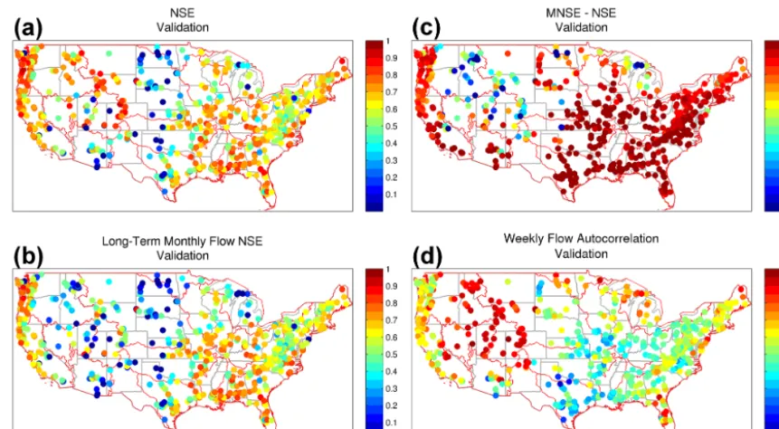
Figure 5. (a) Spatial distribution of NSE, (b) NSE using MNSEs rather than the long-term mean flow, (c) MNSE – NSE for the validation period, and (d) weekly flow autocorrelation.

relative to NSE, particularly in the validation phase (Fig. 5c). This indicates that RMSE as an objective function may not be well suited for model calibration in basins with high flow au-tocorrelation (Kavetski and Fenicia, 2011; Evin et al., 2014). This is confirmed by comparing Fig. 5d to Fig. 5c, basins with large flow autocorrelations (1 week mean flow for ex-ample) generally have lower MNSE scores.

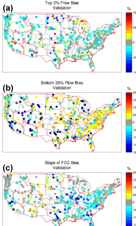
Areas with low-validation NSE and MNSE scores have generally large biases when looking at FDC metrics as well (Fig. 6). Focusing on the high plains, high flow biases of ±50 % are common. Extreme negative low flow biases are also present along the high plains and desert SW along with a general model trend to have large negative FDC slope bi-ases, consistent with a poorly calibrated model. For the 72 % of basins with validation NSE >0.55 (basins with yellow-green to dark red colors in Fig. 6a), there is no noticeable spatial pattern across the CONUS in regard to high flow peri-ods. However, basins with a more pronounced seasonal cycle (e.g., snowpack-dominated watersheds, central west coast) generally have a negative low flow bias, while basins with a smaller seasonal cycle have a positive low flow bias (Fig. 6b). Correspondingly, basins with a pronounced seasonal cycle generally have a near zero or positive slope of the FDC bias, while basins with a smaller seasonal cycle have a negative slope bias (Fig. 6c).

Past applications with similar conceptual snow and hydro-logic modeling systems across the CONUS have shown com-parable spatial performance patterns. Clark et al. (2008) ap-plied many conceptual models to a subset of the MOPEX basin set and found poor performance in arid regions.

Mar-tinez and Gupta (2010), using a monthly water balance model, found the best performance generally along the east coast, most of SE CONUS, and along the west coast with scattered good performance in the Rocky Mountains. They found that many basins along the high plains and north side of the Appalachian Mountains perform poorly. They also note that arid regions have high variability error (variability bias term in KGE – Kling–Gupta efficiency).

4.3 Cumulative performance

Figure 6. (a) Spatial distribution of the high flow bias, (b) low flow bias, and (c) flow duration curve bias for the validation period.

calibration (validation) period total flow bias within 10 % of the observed flow (Fig. 7d). These are expected results when using RMSE for the objective function (Gupta et al., 2009) and reaffirm that our implementation of the SCE calibrates the model properly.

Figure 8 highlights the full split sample approach for cal-ibration following Klemes (1986). It is seen that the calibra-tion and validacalibra-tion statistics give quite similar results regard-less of which time period is used for calibration and vali-dation using the Daymet data. This could indicate that both halves of the data are equally challenging to model with this modeling system. We have also included basin calibrations using only the first 15 years for the Maurer et al. (2002) and NLDAS-II (Xia et al., 2012) data sets. It can be seen that the Daymet forcing provides better model performance overall than both Maurer et al. and NLDAS forcing data. This likely relates to the coarser resolution of the Maurer et

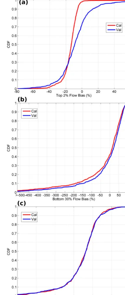
Figure 7. (a) CDFs of the model NSE (solid) for the calibration (red) and validation periods (blue) and NSE using the MNSEs (dark shaded and dashed). CDFs for (b) simulated–observed flow corre-lation in the decomposition of the NSE, (c) for the variance bias in the decomposition of the NSE, and (d) total volume bias in the decomposition of the NSE.

Figure 8. Cumulative density functions for model Nash–Sutcliffe efficiency for the calibration (solid) and validation (dashed) periods using three different forcing data sets (Daymet, Maurer, NLDAS). The Daymet data set was calibrated using the first 15 years (Split 1st) and validated against the remaining data and also calibrated using the last 15 years (Split 2nd) and validated against the initial streamflow data. Maurer and NLDAS calibrations performed using the first 15 years of observed streamflow only.

near-zero total flow bias (Fig. 7). This manifests itself in the simulated hydrograph as underpredicted high flows, gener-ally overpredicted low flows and a more positive slope to the middle portion of the FDC (Fig. 9). It is worth repeating that the goal of this initial application is to provide to community with a benchmark of model performance using well known models, calibration systems and widely used, simple objec-tive functions, thus the use of RMSE.

4.4 Error characteristics

When examining fractional error statistics for the basin set, 15 basins have single days that contribute at least half the total squared error (potential outlier basins), whereas at the median, the largest error day contributes 8.3 % of the total squared error for the median basin (Fig. 10). The fractional error contribution for the 10, 100 and 1000 largest error days for the median basin are 33, 70 and 96 % of the total squared error respectively. This indicates that for nearly all basins, there are 100 or fewer points that drive the RMSE and there-fore optimal model parameters. This type of analysis can be undertaken for any objective function to identify the most influential points and allow for more in-depth examination of forcing data, streamflow records, and calibration strate-gies (i.e., Kavetski et al., 2006; Vrugt et al., 2008; Beven and Westerberg, 2011; Beven et al., 2011; Kauffeldt et al., 2013), or if different model physics are warranted.

The spatial distribution of fractional error contributions show that the issue of model performance being explained

Figure 9. (a) CDFs for model high flow bias for the calibration (red) and validation periods (blue), (b) model low flow bias, and (c) model flow duration curve slope bias.

Figure 10. Fractional contribution of the total squared error for the 1, 10, 100, 1000 largest error days. The box plots represent the 671 basins with the blue area defining the interquartile range, the whiskers representing reasonable values and the red crosses denot-ing outliers. The median is given by the red horizontal line with the notch in the box denoting the 95 % confidence interval of the median value.

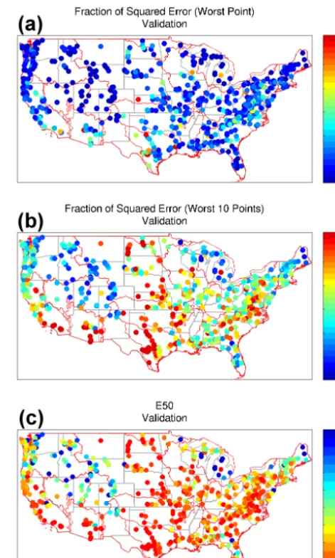
interspersed throughout the record. Basins with significant snowpack tend to have lower error contributions from the largest error days (Fig. 11a, b). The E50 metric highlights mean peak snow water equivalent (SWE) and frequent pre-cipitation basins as well. These regions contain and order of magnitude more days than the high plains and desert SW, giving insight into how representative of the entire stream-flow time series the optimal model parameter set really is.

Additionally, ranking the basins using their fractional er-ror characteristics provides a similar insight. As the aridity index increases, the fractional error contribution increases for basins with little to no mean peak SWE. For basins with significant SWE, the fractional error contribution decreases with increasing aridity (Fig. 12). Alternatively, for a given aridity index the fractional error contribution forNdays will decrease with increasing SWE. This dynamic arises because more arid basins with SWE produce a relatively greater pro-portion of their runoff from snowmelt, without intervening rainfall. This implies that the optimized model produces a more uniform error distribution with less heteroscedacity in basins with more SWE. Moreover, as the fractional error contribution for the 10 largest error days increases, model NSE generally decreases in the validation phase (Fig. 13). This indicates fractional error metrics are related to overall model performance and that calibration methods to reduce extreme error days should improve model performance. This is not unexpected due to the fact that the residuals from an RMSE-type calibration are heteroscedastic. Arid basins typ-ically have few high flow events, which are generally subject

Figure 11. (a) Spatial distribution of the fractional contribution of total squared error for the largest day during the validation period, the (b) 10 largest error days, and (c) the number of days contributing 50 % of the total objective function error, E50.

to larger errors when minimizing the RMSE. Using advanced calibration methodologies that account for heteroscedasticity (Kavetski and Fenicia, 2011; Evin et al., 2014) may produce improved calibrations for arid basins in this basin set and pro-vide different insights into model behavior using this type of analysis.

4.5 Limitations and uncertainties

Figure 12. Ranked fractional squared error contribution for the 100 largest error days for the 671 basins versus the aridity index with mean maximum SWE shaded. Each dot represents a 32-basin bin defined by the rank of the fractional error contribution for the 100 largest error days for all basins. The dashed vertical black lines de-note the 95 % confidence interval for the mean of the fractional error contribution for a given bin.

the Pacific northwest, it is seen that several basins along the west coast have low outlier NSE scores. Tracing this unex-pected result, we find the Daymet forcing data available for those basins has a negative temperature bias, preventing mid-winter rain and melt episodes in the modeling system, iden-tifying scope for improvement in the Daymet forcing. More-over, winter periods of observed precipitation and streamflow rises coincide with subzeroTmaxin the Daymet data set, also suggesting areas to improve the Daymet forcing. The large-sample of basins in this region (91) allowed for identification of the outlier basins and the underlying causes.

This may also limit interpretation of these results and other large-sample hydrologic studies. As noted by Gupta et al. (2014), large-sample hydrology requires a tradeoff be-tween breadth and depth. The lack of depth may inhibit dis-covery and identification of all data quality issues and the underlying causes of outliers in any analysis (e.g., Fig. 13). Explanation of these outliers is sometimes difficult and not complete in the initial development and analysis due to the lack of familiarity with specific basins and any ing or validation data peculiarities. However, providing forc-ing data, model parameters and model output permits ad-ditional focused studies and helps reduce these limitations. Additional prescreening using the methods of Martinez and Gupta (2011) can also help identify outliers due to data qual-ity issues and help identify basins and regions where model physics errors are present.

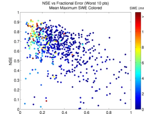
Figure 13. Nash–Sutcliffe efficiency versus the fractional error of the 10 largest error days for the validation period for all basins with basin mean peak snow water equivalent (mm) colored.

5 Summary and discussion

Most hydrologic studies focus in detail on a small number of watersheds, providing comprehensive but highly local in-sights, and may be limited in their ability to inform gen-eral hydrologic concepts applicable across regions (Gupta et al., 2014). To facilitate large-sample hydrologic studies, large-sample basin data sets and corresponding benchmarks of model performance using standard methodology across all basins need to be freely available to the community. To that end, we have compiled a community data set of daily forcing and streamflow data for 671 basins and provide a benchmark of performance using a widely used conceptual a hydrologic modeling and calibration scheme over a wide range of con-ditions.

the data set, which contains forcing and streamflow data ob-tained by consistent methodology and retains outlier basins, makes it a notable resource for these and other future large-sample watershed-scale hydrologic analysis efforts.

This data set and the applications presented are made available to the community (see http://ral.ucar.edu/projects/ hap/flowpredict/subpages/modelvar.php or http://dx.doi.org/ 10.5065/D6MW2F4D).

Acknowledgements. This work is funded by the US Army Corps of Engineers Climate Preparedness and Resilience Programs and the US Department of the Interior Bureau of Reclamation. The authors would like to thank the USGS Modeling of Watershed Systems (MoWS) group, specifically for providing technical support and the national geospatial fabric data to generate all the basin spatial configurations. We would also like to thank Jordan Read and Tom Kunicki of the USGS Center for Integrated Data Analytics for their help with the USGS Geodata Portal.

Edited by: S. Archfield

References

Allen, R. G., Pereira, L. S., Raes, D., and Smith, M.: Crop evapo-transpiration: guidelines for computing crop water requirements. Food and Agriculture Organization of the United Nations, Rome, 15 pp., 1988.

Anderson, E. A.: National Weather Service River Forecast System – Snow accumulation and ablation model. NOAA Technical Mem-orandum, NWS, HYDRO-17, US Department of Commerce, Sil-ver Spring, MD, 217 pp., 1973.

Anderson, E. A.: Calibration of conceptual hydrologic models for use in river forecasting. NOAA Technical Report, NWS 45, Hy-drology Laboratory, Silver Spring, MD, 2002.

Anderson, R. M., Koren, V. I., and Reed, S. M.: Using SSURGO data to improve Sacramento Model a priori parameter estimates, J. Hydrol., 320, 103–116, 2006.

Andreassian, V., Oddos, A., Michel, C., Anctil, F., Perrin, C., and Loumange, C.: Impact of spatial aggregation of inputs and pa-rameters on the efficiency of rainfall-runoff models: A theoret-ical study using chimera watersheds, Water Resour. Res., 40, W05209, doi:10.1029/2003WR002854, 2004.

Beldring, S., Engeland, K., Roald, L. A., Sælthun, N. R., and Voksø, A.: Estimation of parameters in a distributed precipitation-runoff model for Norway, Hydrol. Earth Syst. Sci., 7, 304–316, doi:10.5194/hess-7-304-2003, 2003.

Beven, K. and Westerberg, I.: On red herrings and real herrings: dis-information and dis-information in hydrological inference, Hydrol. Process., 25, 1676–1680, 2011.

Beven, K., Smith, P. J., and Wood, A.: On the colour and spin of epistemic error (and what we might do about it), Hy-drol. Earth Syst. Sci., 15, 3123–3133, doi:10.5194/hess-15-3123-2011, 2011.

Blodgett, D. L., Booth, N. L., Kunicki, T. C., Walker, J. L., and Viger, R. J.: Description and testing of the geo data portal: A data integration framework and web processing services for

environ-mental science collaboration. US Geological Survey, Open-File Report 2011-1157, 9 pp., Middleton WI, USA, 2011.

Burnash, R. J. C.: The NWS River Forecast System – Catchment model, in: Computer Models of Watershed Hydrology, edited by: Singh, V. P., 311–366, Water Resources Publications, Highlands Ranch, Colo, 1995.

Burnash, R. J. C., Ferral, R. L., McGuire, R. A.: A generalized streamflow simulation system conceptual modeling for digital computers, US Department of Commerce National Weather Ser-vice and State of California Department of Water Resources, 1973.

Clark, C. O.: Storage and the unit hydrograph. Proc. Am. Soc. Civ. Eng., 9, 1333–1360, 1945.

Clark, M. P., Slater, A. G., Rupp, D. E., Woods, R. A., Vrugt, J. A., Gupta, H. V., Wagener, T., and Hay, L. E.: Framework for Un-derstanding Structural Errors (FUSE): A modular framework to diagnose differences between hydrologic models, Water Resour. Res., 44, W00B02, doi:10.1029/2007WR006735, 2008. Dooge, J. C. I.: A general theory of the unit hydrograph, J. Geophys.

Res., 64, 241–256, 1959.

Duan, Q., Sorooshian, S., and Gupta, V. K.: Effective and efficient global optimization for conceptual rainfall-runoff models, Water Resour. Res., 28, 1015–1031, 1992.

Duan, Q., Gupta, V. K., and Sorooshian, S.: A shuffled complex evo-lution approach for effective and efficient optimization, J. Opti-miz. Theor. Appl., 76, 501–521, 1993.

Duan, Q., Sorooshian, S., and Gupta, V. K.: Optimal use of the SCE-UA global optimization method for calibrating watershed mod-els, J. Hydrol., 158, 265–284, 1994.

Duan, Q., Schaake, J., Andreassian, V., Franks, S., Goteti, G., Gupta, H. V., Gusev, Y. M., Habets, F., Hall, A., Hay, L., Houge, T., Huang, M., Leavesley, G., Liang, X., Nasonova, O. N., Noil-han, J., Oudin, L., Sorooshian, S., Wagener, T., and Wood, E. F.: Model Parameter Estimation Experiment (MOPEX): An overview of science strategy and major results from the second and third workshops, J. Hydrol., 320, 3–17, 2006.

Durre, I., Menne, M. J., and Vose, R. S.: Strategies for evaluat-ing quality assurance procedures, J. Appl. Meteor. Climatol., 47, 1785–1791, doi:10.1175/2007JAMC1706.1, 2008.

Durre, I., Menne, M. J., Gleason, B. E., Houston, T. G., and Vose, R. S.: Comprehensive Automated Quality Assurance of Daily Sur-face Observations, J. Appl. Meteor. Climatol., 49, 1615–1633, doi:10.1175/2010JAMC2375.1, 2010.

Evin, G., Thyer, M., Kavetski, D., McInerney, D., and Kuczera, G.: Comparison of joint versus postprocessor approaches for hydro-logical uncertainty estimation accounting for error autocorrela-tion and heteroscedasticity, Water Resour. Res., 50, 2350–2375, doi:10.1002/2013WR014185, 2014.

Falcone, J. A.: GAGES-II: Geospatial Attributes of Gages for Evaluating Streamflow. Digital spatial data set 2011, available at: http://water.usgs.gov/GIS/metadata/usgswrd/XML/ gagesII_Sept2011.xml (last access: 10 October 2013), 2011. Falcone. J. A., Carlisle, D. M., Wolock, D. M., and Meador, M. R.:

Garrick, M., Cunnane, C., and Nash, J. E.: A criterion of efficiency for rainfall-runoff models, J. Hydrology, 36, 375–381, 1978. Gupta, H. V., Kling, H., Yilmaz, K. K., and Martinez-Barquero, G.

F.: Decomposition of the mean squared error and NSE perfor-mance criteria: Implications for improving hydrological model-ing, J. Hydrol., 377, 80–91, doi:10.1016/j.jhydrol.2009.08.003, 2009.

Gupta, H. V., Perrin, C., Blöschl, G., Montanari, A., Kumar, R., Clark, M., and Andréassian, V.: Large-sample hydrology: a need to balance depth with breadth, Hydrol. Earth Syst. Sci., 18, 463– 477, doi:10.5194/hess-18-463-2014, 2014.

Jensen, M. E., Burman, R. D., and Allen, R. G.: Evapotranspiration and irrigation water requirements. American Society of Civil En-gineers, ASCE Manual and Reports on Engineering Practice, 332 p., New York, NY, 1990.

Jin, S., Yang, L., Danielson, P., Homer, C., Fry, J., and Xian, G.: A comprehensive change detection method for updating the Na-tional Land Cover Database to circa 2011, Remote Sens. Envi-ron., 132, 159–175, 2013.

Kauffeldt, A., Halldin, S., Rodhe, A., Xu, C.-Y., and Westerberg, I. K.: Disinformative data in large-scale hydrological modelling, Hydrol. Earth Syst. Sci., 17, 2845–2857, doi:10.5194/hess-17-2845-2013, 2013.

Kavetski, D. and Fenicia, F.: Elements of a flexible ap-proach for conceptual hydrological modeling: 2. Application and experimental insights, Water Resour. Res., 47, W11511, doi:10.1029/2011WR010748, 2011.

Kavetski, D., Kuczera, G., and Franks, S. W.: Bayesian analysis of input uncertainty in hydrological modeling: 2. Application, Water Resour. Res., 42, W03407, doi:10.1029/2005WR004376, 2006.

Klemes, V.: Operational testing of hydrological simulation models, Hydrol. Sci. J., 31, 13–24, 1986.

Koren, V. I., Smith, M., Wang, D., and Zhang, Z.: Use of soil prop-erty data in the derivation of conceptual rainfall-runoff model parameters. American Meteorological Society 15th Conference on Hydrology, Long Beach, CA, 103–106, 2000.

Kumar, R., Samaniego, L., and Attinger, S.: Implications of dis-tributed hydrologic model parameterization on water fluxes at multiple scales and locations, Water Resour. Res., 49, 360–379, doi:10.1029/2012WR012195, 2013.

Lins, H. F.: USGS Hydro-Climatic Data Network 2009 (HCDN-2009), US Geological Survey, Fact Sheet 2012-3047, Reston VA, USA, 2012.

Livneh, B. and Lettenmaier, D. P.: Multi-criteria parameter estima-tion for the Unified Land Model, Hydrol. Earth Syst. Sci., 16, 3029–3048, doi:10.5194/hess-16-3029-2012, 2012.

Livneh, B. and Lettenmaier, D. P.: Regional parameter estimation for the Unified Land Model, Water Resour. Res., 49, 100–114, doi:10.1029/2012WR012220, 2013.

Livneh, B., Rosenberg, E. A., Lin, C., Nijssen, B., Mishra, V., An-dreadis, K. M., Maurer, E. P., and Lettenmaier, D. P.: A Long-Term Hydrologically Based Dataset of Land Surface Fluxes and States for the Conterminous United States: Update and Ex-tensions, J. Climate, 26, 9384–9392, doi:10.1175/JCLI-D-12-00508.1, 2013.

Lohmann, D., Mitchell, K. E., Houser, P. R., Wood, E. F., Schaake, J. C., Robock, A., Cosgrove, B. A., Sheffield, J., Duan, Q., Luo, L., Higgins, R. W., Pinker, R. T., and Tarpley, J. D.: Streamflow

and water balance intercomparisons of four land surface models in the North American Land Data Assimilation System project, J. Geophys. Res., 109, D07S91, doi:10.1029/2003JD003517, 2004. Martinec, J. and Rango, A.: Merits of statistical criteria for the per-formance of hydrological models, Water Resour. B., 25, 421– 432, 1989.

Martinez, G. and Gupta, H. V.: Toward improved identifi-cation of hydrologic models: A diagnostic evaluation of the “abcd” monthly water balance model for the conter-minous United States, Water Resour. Res., 46, W08507, doi:10.1029/2009WR008294, 2010.

Martinez, G. and Gupta, H. V.: Hydrologic consistency as a basis for assessing complexity of monthly water balance models for the continental United States, Water Resour. Res., 47, W12540, doi:10.1029/2011WR011229, 2011.

Maurer, E. P., Wood, A. W., Adam, J. C., Lettenmaier, D. P., and Nijssen, B.: A long-term hydrologically-based data set of land surface fluxes and states for the conterminous United States, J. Climate, 15, 3237–3251, 2002.

Menne, M. J., Williams Jr., C. N., and Vose, R. S.: The U.S. Historical Climatology Network monthly temperature data, version 2, Bull. Am. Meteor. Soc., 90, 993–1007, doi:10.1175/2008BAMS2613.1, 2009

Menne, M. J., Williams, C. N., and Palecki, M. A.: On the reliability of the U.S. surface temperature record, J. Geophys. Res., 115, D11108, doi:10.1029/2009JD013094, 2010.

Merz, R. and Bloschl, G.: Regionalization of catchment model pa-rameters, J. Hydrol., 287, 95–123, 2004.

Mizukami, N., Koren, V., Smith, M., Kingsmill, D., Zhang, Z., Cos-grove, B., and Cui, Z.: The impact of precipitation type dis-crimination on hydrologic simulation: Rain-snow partitioning derived from HMT-West radar-detected brightband height ver-sus surface temperature data, J. Hydrometeorol., 14, 1139–1158, doi:10.1175/JHM-D-12-035.1, 2013.

Morton, F. I.: Operational estimates of actual evapotranspiration and their significance to the science and practice of hydrology, J. Hy-drol., 66, 1–76, 1983.

Nash, J. E.: The form of the instantaneous unit hydrograph, Interna-tional Association of Scientific Hydrology Publication, 45, 114– 121, Toronto ON, CA, 1957.

Nash, J. E. and Sutcliffe, J. V.: River flow forecasting through con-ceptual models. Part I: A discussion of principles, J. Hydrol., 10, 282–290, doi:10.1016/0022-1694(70)90255-6, 1970.

Nathan, R. J. and McMahon, T. A.: The SFB model, Part I – Vali-dation of fixed model parameters, Civil Eng. Trans., CE32, 157– 161, 1990.

Nester, T., Kirnbauer, R., Gutknecht, D., and Bloschl, G.: Climate and catchment controls on the performance of regional flood sim-ulations, J. Hydrol., 402, 340–356, 2011.

Nester, T., Kirnbauer, R., Parajka, J., and Bloschl, G.: Evaluating the snow component of a flood forecasting model, Hydrol. Res., 43, 762–779, 2012.

Oubeidillah, A. A., Kao, S.-C., Ashfaq, M., Naz, B. S., and Tootle, G.: A large-scale, high-resolution hydrological model parameter data set for climate change impact assessment for the contermi-nous US, Hydrol. Earth Syst. Sci., 18, 67–84, doi:10.5194/hess-18-67-2014, 2014.

complementary model parameterizations, Water Resour. Res., 42, W07410, doi:10.1029/2005WR004636, 2006.

Oudin, L., Kay, A. L., Andreassian, V., and Perrin, C.: Are seemingly physically similar catchments truly hy-drologically similar?, Water Resour. Res., 46, W11558, doi:10.1029/2009WR008887, 2010.

Perrin, C., Michel, C., and Andreassian, V.: Does a large num-ber of parameters enhance model performance? Comparative assessment of common catchment model structures on 429 catchments, J. Hydrol., 242, 275–301, doi:210.1016/S0022-1694(1000)00393-00390, 2001.

Pokhrel, P. and Gupta, H. V.: On the use of spatial regularization strategies to improve calibration of distributed watershed models, Water Resour. Res., 46, W01505, doi:10.1029/2009WR008066, 2010.

Priestly, C. H. B. and Taylor, R. J.: On the assessment of surface heat flux and evaporation using large-scale parameters, Mon. Weather Rev., 100, 81–82, 1972.

Samaniego, L., Bardossy, A., and Lumar, R.: Streamflow prediction in ungauged catchments using copula-based dissimilarity measures, Water Resour. Res., 46, W02506, doi:10.1029/2008WR007695, 2010.

Schaake, J., Cong, S., Duan, Q.: U.S. MOPEX data set. Report UCRL-JRNL-221228, Lawrence Livermore National Labora-tory, Livermore CA, USA, available at: https://e-reports-ext.llnl. gov/pdf/333681.pdf (last access: 10 September 2014), 2006. Schaefli, B., Hingray, B., Niggli, M., and Musy, A.: A conceptual

glacio-hydrological model for high mountainous catchments, Hydrol. Earth Syst. Sci., 9, 95–109, doi:10.5194/hess-9-95-2005, 2005.

Schaefli, B. and Gupta, H. V.: Do Nash values have value?, Hydrol. Process., 21, 2075–2080, doi:10.1002/hyp.6825, 2007.

Schlosser, C. A., Slater, A. G., Robock, A., Pitman, A. J., Vinnikov, K. Y., Henderson-Sellers, A., Speranskaya, N. A., Mitchell, K., and the PILPS 2(d) contributors: Simulations of a boreal grassland hydrology at Valdai, Russia: PILPS phase 2(d), Mon. Weather Rev., 128, 301–321, 2000.

Sherman, L. K.: Streamflow from rainfall by the unit graph method, Eng. News Rec., 108, 501–505, 1932.

Shi, X., Wood, A. W., and Letenmaier, D. P.: How essential is hy-drologic model calibration to seasonal streamflow forecasting?, J. Hydrometeorol., 9, 1350–1363, 2008.

Shuttleworth, W. J. and Calder, I. R.: Has the Priestly-Taylor equa-tion any relevance to forest evaporaequa-tion?, J. Appl. Meteorol., 18, 639–646, 1979.

Slack, J. R. and Landwehr, J. M.: Hydro-Climatic Data Network (HCDN): A US Geological Survey streamflow data set for the United States for the study of climate variations, 1874–1988, US Geological Survey, Open-File Report 92-129, Reston VA, USA, 1992.

Sorooshian, S., Duan, Q., and Gupta, V. K.: Calibration of concep-tual rainfall-runoff models using global optimization: application to the Sacramento soil moisture accounting model, Water Resour. Res., 29, 1185–1194, 1993.

Thornton, P. E. and Running, S. W.: An improved algorithm for estimating incident daily solar radiation from measurements of temperature, humidity and precipitation, Agr. Forest Meteorol., 93, 211–228, 1999.

Thornton, P. E., Running, S. W., and White, M. A.: Generating surfaces of daily meteorological variables over large regions of complex terrain, J. Hydrol., 190, 214–251, doi:10.1016/S0022-1694(96)03128-9, 1997.

Thornton, P. E., Hasenauer, H., and White, M. A.: Simultaneous estimation of daily solar radiation and humidity from observed temperature and precipitation: An application over complex ter-rain in Austria, Agr. Forest Meteorol., 104, 255–271, 2000. Thornton, P. E., Thornton, M. M., Mayer, B. W., Wilhelmi, N., Wei,

Y., and Cook, R. B.: Daymet: Daily surface weather on a 1 km grid for North America, 1980–2012, available at: http://daymet. ornl.gov/ (last access: 15 July 2013) from Oak Ridge National Laboratory Distributed Active Archive Center, Oak Ridge, Ten-nessee, USA, 2012.

Viger, R. J.: Preliminary spatial parameters for PRMS based on the Geospatial Fabric, NLCD2001 and SSURGO, US Geologi-cal Survey, doi:10.5066/F7WM1BF7, 2014.

Viger, R. J. and Bock, A.: GIS Features of the Geospatial Fab-ric for National Hydrologic Modeling, US Geological Survey, doi:10.5066/F7542KMD, 2014.

Vrugt, J. A., ter Braak, C. J. F., Clark, M. P., Hyman, J. M., and Robinson, B. A.: Treatment of input uncertainty in hy-drologic modeling: Doing hydrology backward with Markov chain Monte Carlo simulation, Water Resour. Res., 44, W00B09, doi:10.1029/2007WR006720, 2008.

Xia, Y., Mitchell, K., Ek, M., Sheffield, J., Cosgrove, B., Wood, E., Luo, L., Alonge, C., Wei, H., Meng, J., Livneh, B., Letten-maier, D., Koren, V., Duan, Q., Mo, K., Fan, Y., and Mocko, D.: Continental-scale water and energy flux analysis and val-idation for the North American Land Data Assimilation Sys-tem project phase 2 (NLDAS-2): 1. Intercomparison and ap-plication of model products, J. Geophys. Res., 117, D03109, doi:10.1029/2011JD016048, 2012.

Yang, D., Goodison, B. E., Metcalfe, J. R., Golubev, V. S., Bates, R., Pangburn, T., and Hanson, C. L.: Accuracy of NWS 8” stan-dard nonrecording precipitation gauge: Results and application of WMO intercomparison, J. Atmos. Ocean. Technol., 15, 54– 68, 1998.

Yilmaz, K. K., Gupta, H. V., and Wagener, T.: A process-based di-agnostic approach to model evaluation: Application to the NWS distributed hydrologic model, Water Resour. Res., 44, W09417, doi:10.1029/2007WR006716, 2008.

Zhang, Z., Koren, V., Reed, S., Smith, M., Zhang, Y., Moreda, F., and Cosgrove, B.: SAC-SMA a priori parameter differences and their impact on distributed hydrologic model simulations, J. Hy-drol., 420–421, 216–227, 2012.