https://doi.org/10.5194/hess-21-4959-2017 © Author(s) 2017. This work is distributed under the Creative Commons Attribution 3.0 License.
Consistent initial conditions for the Saint-Venant equations
in river network modeling
Cheng-Wei Yu1, Frank Liu2, and Ben R. Hodges1
1Center for Water and the Environment, The University of Texas at Austin, 10100 Burnet Road, Bldg. 119, Austin, TX 78712, USA
2IBM Research Austin, 11501 Burnet Road, Austin, TX 78758, USA Correspondence to:Cheng-Wei Yu ([email protected]) Received: 27 February 2017 – Discussion started: 3 April 2017
Revised: 26 June 2017 – Accepted: 9 August 2017 – Published: 29 September 2017
Abstract. Initial conditions for flows and depths (cross-sectional areas) throughout a river network are required for any time-marching (unsteady) solution of the one-dimensional (1-D) hydrodynamic Saint-Venant equations. For a river network modeled with several Strahler orders of tributaries, comprehensive and consistent synoptic data are typically lacking and synthetic starting conditions are needed. Because of underlying nonlinearity, poorly defined or inconsistent initial conditions can lead to convergence problems and long spin-up times in an unsteady solver. Two new approaches are defined and demonstrated herein for computing flows and cross-sectional areas (or depths). These methods can produce an initial condition data set that is consistent with modeled landscape runoff and river ge-ometry boundary conditions at the initial time. These new methods are (1) the pseudo time-marching method (PTM) that iterates toward a steady-state initial condition using an unsteady Saint-Venant solver and (2) the steady-solution method (SSM) that makes use of graph theory for initial flow rates and solution of a steady-state 1-D momentum equation for the channel cross-sectional areas. The PTM is shown to be adequate for short river reaches but is significantly slower and has occasional non-convergent behavior for large river networks. The SSM approach is shown to provide a rapid solution of consistent initial conditions for both small and large networks, albeit with the requirement that additional code must be written rather than applying an existing un-steady Saint-Venant solver.
1 Introduction 1.1 Motivation
discussed herein) may not be as sensitive to consistent initial conditions.
Saint-Venant equation modeling arguably dates from Preissmann’s seminal work (Preissmann, 1961; Preissmann and Cunge, 1961), followed by decades of advances in tech-niques and applications (Cunge, 1974; Ponce et al., 1978; Cunge et al., 1980; Abbott et al., 1986; Zhao et al., 1996; Sanders, 2001; Pramanik et al., 2010). These models focused on hydraulics of short river reaches or main stem rivers that are easy to initialize for flow and depth. It is only recently that the solvers for large river networks have become practical (Hodges, 2013; Liu and Hodges, 2014), and it is with large networks that initial conditions are problematic. Indeed, ini-tial conditions and associated spin-up problems have been re-cently acknowledged and investigated for hydrological mod-els (e.g., Ajami et al., 2014) but without consideration of a separate river network model. Work by Seck et al. (2015) and Rahman and Lu (2015) show that hydrological model spin-up computational times could be significant and were dominated by the selected initial hydrological conditions.
Our experience with Saint-Venant river network modeling is that simple approaches to initial conditions often cause lo-calized numerical instabilities, slow convergence of the time-marching numerical solution, and long model spin-up times. Herein, we investigate the initial condition problem for a Saint-Venant river network model for a given set of inflows from a hydrological model.
1.2 Synthetic vs. observed initial conditions
Model spin-up time is completed when the effects of initial conditions cannot be observed in the model results. Thus, by definition, the initial conditions cannot affect the unsteady solution beyond spin-up time. It follows that initial condi-tions are irrelevant to the quality of the time-marching simu-lation and are only important in how they affect the spin-up duration. We can imagine a “perfect” set of initial conditions with zero spin-up time, which would require initial flows and depths consistent with (i) the actual unsteady behavior prior to the model start time and (ii) the model boundary condi-tions; the latter includes both the bathymetric model for the river channels and the coupled hydrological model providing runoff and baseflows. Such perfect initial conditions are prac-tically unattainable due to the sparsity of synoptic flow/depth data as well as unavoidable uncertainty and errors in both bathymetric and hydrological models. Another way to think of this is that perfect initial conditions also require perfect boundary conditions (perfect bathymetry and hydrology), or else some spin-up time is required to wash out inconsisten-cies. In general, the spin-up time will be affected by how far the initial conditions are from the theoretical perfect condi-tions.
The key point is that the exact observed river initial condi-tions (if such were available throughout a network) will not eliminate or necessarily reduce spin-up time if the observed
data are inconsistent with the model boundary conditions. Similarly, interpolations of sparse synoptic data will not be a priori consistent with the boundary conditions and thus can-not eliminate spin-up time. Inconsistency is a critical con-cept: the mismatches between the initial conditions and the boundary conditions can lead to unrealistic destabilizing im-pulses in time marching the SVE solution. Such imim-pulses can require extensive spin-up time to damp their effects. An ex-treme example is a high runoff rate into an almost dry stream that can cause a Gibbs phenomenon at a wave front and nega-tive values for the computed cross-sectional area (Lax, 2006; Kvoˇcka et al., 2015; Yang et al., 2012). Although several studies show such numerical discontinuities can be resolved (Kazolea and Delis, 2013; Caleffi et al., 2003; Liang et al., 2006), the high computational cost of damping or resolving is a burden (Kvoˇcka et al., 2015) that seems unnecessary dur-ing spin-up since it cannot affect the time-marchdur-ing results.
We argue that the primary goal of initial conditions is pro-viding consistency with the boundary conditions to allow smooth, convergent spin-up of an unsteady solver. This task can be accomplished with synthetic initial conditions that are independent of observations. The only practical discrimina-tors between using observed and synthetic initial conditions are (i) the effort required to prepare the initial condition data and (ii) the length of spin-up time.
As demonstrated herein, consistent synthetic initial con-ditions can be readily generated for even large complex net-works – a task that is daunting for interpolation/extrapolation of sparse synoptic observations. Indeed, developing consis-tent synthetic initial conditions only requires the channel ge-ometry and hydrological model that are used for the SVE time marching, supplemented by a steady-state SVE solver (Sect. 2.3). In contrast, interpolation/extrapolation of synop-tic data requires analysis of the data locations and model ge-ometry, which is likely to require customization for each river network.
1.3 Initial condition approaches
Approaches for specifying initial conditions for the SVE can be grouped into three main categories: (i) a “synoptic start” applying an interpolated/extrapolated set of sparse observa-tional data, (ii) a “cold start” with initial flow rates and flow depths prescribed either as zero (e.g., Chau and Lee, 1991) or from some analytical values, e.g., mean annual flows and depths, and (iii) a “steady-state” start, which we describe herein. The metric for evaluating initial conditions is not how well they reflect available real-world observations but how effective they are in efficiently providing a consistent set of initial conditions.
Based on our discussion above, the first approach (synop-tic start) is unlikely to be efficient for SVE initial conditions in a large river network due to inconsistencies between obser-vations and model boundary conditions as well as inconsis-tencies caused by interpolating/extrapolating sparse observa-tions throughout a network. There are no proven approaches to analyzing consistency and melding observations to hydro-logical model runoff, so the river network model spin-up will be subject to random inconsistencies and instabilities that can delay or prevent convergence.
The second approach, a cold start, provides innumerable possible ways to create initial conditions. For example, mean annual flows and depths (e.g., from the NHDPlus data in the US) can provide a smooth and consistent set of flows and elevations throughout a network. Although such cold start initial conditions can be internally consistent, they may be far from the flows/depths implied by the initial hydrological forcing. For example, a river network model that is started with mean annual values would be substantially in error if the initial hydrological inflows were from the monsoon season. As a result of inconsistencies between the selected cold start values and the hydrological inflows, a cold start can require extensive spin-up time to dilute or wash out the error. Indeed, the spin-up time dominated the computational time for the large SVE networks that we previously modeled in Liu and Hodges (2014) when we used a cold start with mean annual values. It might be possible to design a cold start approach that is consistent with the hydrological inflows; however, we suspect that any such approach is likely to be merely a variant of the steady-state approach discussed herein.
Herein, we investigate the third approach, steady-state ini-tial conditions, as a preferred method for iniini-tializing a large river network model. With this idea, a set of consistent ini-tial conditions is one that satisfies both thet=0 hydrological forcing and the steady-state Saint-Venant equations att=0. That is, we know that we cannot match the unsteady SVE at
t=0 as we cannot perfectly know the time-varying nonlin-ear effects before the model starts (unless, of course, we run a model for the prior period, which would be simply time shifting the initial condition problem). The steady-state ap-proach has the advantage of providing flows and depths that are consistent across the entire network with all the boundary
conditions (inflows and channel geometry) as well as tent with the nonlinear governing equations. These consis-tencies eliminate destabilizing impulses otherwise caused by mismatches between the flow/depth in a river reach and the runoff, so subsequent time marching of the unsteady solu-tion is smooth. Furthermore, the steady-state solusolu-tion is the closest available proxy to the unknown unsteady solution at
t=0, so this approach should minimize the spin-up time re-quired to reach an unsteady time march that is independent of the initial conditions.
1.4 Overview
Herein, we present an efficient approach to establishing a set of steady-state conditions that provides a consistent and smooth starting point for time marching an unsteady Saint-Venant simulation. A full model initialization problem has two parts: (i) determining a set of flows and water surface elevations that are consistent steady solutions of the SVE for starting an unsteady solver and (ii) determining the spin-up time needed to ensure errors in the initial conditions are washed out of the unsteady solution. The second problem is highly dependent on the network characteristics and the par-ticular flow and boundary conditions during spin-up, so for brevity, this work deals quantitatively with solving the first problem and then illustrates the effects on the second prob-lem.
2 Methods
2.1 Saint-Venant equations
re-lationships). The equation set can be written as
∂A ∂t +
∂Q
∂x =ql (1)
∂Q ∂t +
∂ ∂x
Q2
A
+gA∂h
∂x=gA(S0−Sf), (2)
where boundary conditions are the local channel bottom slope (S0) and the local lateral net inflow (ql), the latter rep-resenting both inflows from the landscape and outflows to groundwater. Auxiliary equations for h=h(A)are derived from river cross-section data. The Chezy–Manning equation can be used to provide the friction slope as
ASf=en
2Q2F, (3)
whereen is the standard Manning’snroughness coefficient andF is a convenient equivalent friction geometry (Liu and Hodges, 2014), which subsumes the conventional hydraulic radius (Rh) using a definition of
F = 1
AR4h/3 =
P4 A7
1/3
, (4)
whereP =P (A)is the wetted perimeter and Rh=AP−1. Note that Eq. (4) fixes a typographical error in Eq. (10) of Liu and Hodges (2014) and Eq. (3.55) of Hodges and Liu (2014). Required boundary conditions for the unsteady Saint-Venant solution are ql(t ) for each stream segment, Qbc(t ) at the
furthest upstream node (headwater) in river branches with a Strahler order of 1, and h with an h(A) relationship at the downstream boundary (assumed subcritical). The time-marching unsteady solution requires initial conditions for (Q, A), which can also be given as (Q, h) with A=A(h). Implementation details of the unsteady solver used herein can be found in Liu and Hodges (2014) and Liu (2014). 2.2 Pseudo time-marching approach
The most obvious approach for finding steady-state initial conditions is to time march an unsteady solver until a steady state is achieved. That is, we apply the unsteady solver with time-invariant boundary conditions ofql(t )=ql(0)and
Qbc(t )=Qbc(0)fort0≤t <0 wheret0is our pseudo time start andt=0 is the time for which we want a set of initial conditions. We call this the pseudo time-marching method (PTM). The initial condition for PTM is a set ofQ(t0)and
A(t0)for each stream segment (e.g., some cold start method as described above). At first glance, the logic here might seem circular: we are trying to solve for initial condition set {Q(0), A(0)}of the unsteady model and PTM requires specifying {Q(t0), A(t0)}. This begs the question as to why PTM should be used rather than simply applying a cold start of the unsteady solver withQ(0)=Q(t0)andA(0)=A(t0). The answer is that the key difference between the PTM us-ingQ(t0)andA(t0)and a cold start of the unsteady solver
with the same values is that the former has time-invariant boundary conditions while the latter’s are time varying. Thus, an unsteady solver with time-varying boundary conditions is trying to take an inconsistent starting condition and converge it to a moving target. In contrast, the PTM takes the incon-sistent starting conditions and attempts to converge them to a time-invariant target, which is more likely to be successful. However, the PTM does not a priori ensure consistency be-tween theQ(t0)andA(t0)starting conditions and thet=0 boundary conditions. It follows that PTM performance can be subject to the same type of problems as a cold start de-pending on the choice ofQ(t0)andA(t0)and the skill of the modeler in their selection. In Sect. 4.5, we show that PTM typically has problems for large river systems with complex geometry because the complexity of selecting a reasonable set of{Q(t0), A(t0)}to ensure convergence.
The PTM is outlined as Algorithm 1. A user-selected pa-rameter () is used as a threshold tolerance value for declar-ing convergence to the steady state. A typical choice of the toleranceis the square root of the computer hardware tol-erance. For example, on a 64-bit Intel architecture, the hard-ware tolerance for a double precision floating point floating number is 2.2204×10⁻¹⁶, which means a good choice of
is 1.4901×10⁻⁸. As a practical matter, of 10−6 or even 10−4 is likely to be sufficient for initial conditions; that is, as further spin-up time is still required to dilute initial con-dition errors, the convergence needs only to be sufficient for consistency across the network. The method can use a time-step size that is either constant or varying, with an automatic reduction in step size when convergence is not achieved in a given time step (Liu and Hodges, 2014). To avoid infinite runtimes for non-convergent behavior (e.g., due to instabili-ties developed with inconsistent starting conditions), the so-lution is terminated (failure to converge) in Algorithm 1 after the user-selectedNmaxiterations. The starting conditions for
{Q(t0), A(t0)}are discussed in Appendix A. 2.3 Steady-solution method
The PTM approach (above) results in a steady solution of the unsteady Saint-Venant equations that satisfies both mo-mentum and continuity for time-invariantql(0)andQbc(0)
boundary conditions in the unsteady solver. However, we can achieve a similar effect more directly by writing a steady-state version of the Saint-Venant equations as
∂Q
∂x =ql (5)
∂ ∂x
Q2
A
+gA∂h
∂x=gA(S0−Sf). (6)
A key point, implied by Eq. (5), is that the spatial gradient of steady-stateQover a stream segment is entirely due to the lateral inflow (ql) without any influence ofA. It follows that for steadyql andQbc boundary conditions, the flow in the
Algorithm 1Pseudo time-marching method
1: procedurePSEUDOTIMEMARCHING (Aini,Qini,,Nmax)
{Aini,Qini: initial guesses ofAandQ;: tolerance;Nmax:
max-imal iteration number} 2: A←Aini
3: Q←Qini
4: i←0 5: t0←0
6: fori=1 toNmaxdo
7: Solve SVE at time pointtiusing unsteady method
8: Compute error:e←Qt−Qt−1 +
At−At−1
9: if e < then
10: return Success
11: end if
12: ti+1←ti+1ti
13: i←i+1 14: end for
15: return Failure
16: end procedure
sum of all theQjfor all thej connected reaches of Strahler
order Sj<Si. That is, the steady flow at any point is simply
the sum of all the connected upstreamt=0 boundary con-ditions. The correspondingA(and hence depthh) can then be computed with a numerical partial differential equation (PDE) solution of Eq. (6) for knownQvalues. Note that for large river networks, the natural downstream boundary con-dition is subcritical, which requires specification ofhand the correspondingAas the starting point. We call this a “steady-solution method” (SSM). To look at this from another view-point, ifAis uniform, then Eq. (6) devolves the fundamental equation of gradually varying flow, dE/dx=S0−Sf, where
Eis the specific energy. Thus, the SSM corresponds to using the steady-state flow based on all boundary conditions and solving for surface elevations with a gradually varying flow solution for non-uniform cross sections.
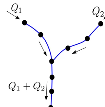
[image:5.612.342.514.63.237.2]To efficiently compute the conservative initialQ through-out the river network, it is useful to apply graph theory as discussed in Hodges and Liu (2014). A river network can be classified as a “direct acyclic graph” (DAG) as a river may split upstream or downstream at a junction, but the flow cannot loop back to a starting point. The connectivity of a DAG can be efficiently computed by applying existing graph methods, such as depth-first search (DFS) or breadth-first search (BFS), which provide simple and efficient approaches to computingQ(0)for each stream segment over an entire network. Note that these methods were designed and named by computer scientists, so “depth” in DFS and “breadth” in BFS do not refer to hydraulics or river geometry but in-stead are jargon referring to the graph network characteris-tics. For simplicity in the present work, we confine ourselves to the subset of DAG systems that are simply connected trees, i.e., where there is never more than a single downstream reach from any junction (as shown in Fig. 1) so that there are
Figure 1.Propagation of flow rateQat a junction.
no uncertainties in flow directions or magnitudes. Extending the method to geometry with multiple downstream reaches (e.g., braiding, canals, deltas) requires additional rules for downstream splitting of flows that are beyond the scope of the present work.
A simple DFS traversal (Cormen et al., 2001) forQ is shown in Algorithm 2. From each headwater node (Qj),
the inflow boundary condition is propagated downstream by adding the value to the downstream node and including any lateralql from the upstream reach (stored inQk). For river
networks, the DFS traversal is highly efficient and requires negligible computational time for river networks of 105 com-putational nodes (e.g., Liu and Hodges, 2014). Based on our experience, the DFS computational costs should be essen-tially trivial for even continental-scale systems of 107nodes. Algorithm 2DFS traversal forQ
1: procedureQTRAVERSAL 2: for allido {initialization} 3: Qi←0
4: end for
5: foreach headwater nodejwith BCQj(t )do
6: Qj←Qj(t=0)
7: k←downstream node of nodej
8: while kis not emptydo
9: Qk←Qk+Qj(t=0)
10: k←downstream node of nodek
11: end while
12: end for
13: return
14: end procedure
After the steadyQifor each stream segment is computed,
Eq. (6) can be solved for the correspondingAi. We discretize
are approximated as
f (x, t )'1
2(fj+1+fj) (7)
∂
∂xf (x, t )'
1
1x(fj+1−fj), (8)
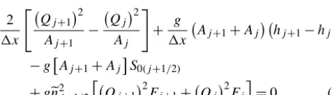
where subscripts indicate a node in the discrete system. Us-ingj+1/2 to represent geometric data that are logically be-tween nodes (i.e., roughnessenandS0), Eq. (6) becomes
2
1x "
Qj+12
Aj+1
− Qj
2 Aj
#
+ g
1x Aj+1+Aj
hj+1−hj
−g
Aj+1+AjS0(j+1/2)
+gen2j+1/2h Qj+12Fj+1+ Qj2Fj
i
=0. (9)
These nonlinear equations are similar to the unsteady dis-crete equations, except thatQfor each computational node is known from the DFS traversal. Newton’s method is used to solve this system for A without linearization, similar to the approach in Liu and Hodges (2014). The SSM re-quires a starting guess forAto solve the steady-state prob-lem. Herein, we use a bisection method with the Chezy– Manning equation for normal depth conditions (discussed in Appendix A). The overall algorithm for SSM is illustrated in Algorithm 3.
Algorithm 3Steady-solution method
1: procedureSTEADYSOULTION 2: Call QTraversal()
3: for allall nodejin networkdo {Initial guess ofA} 4: Call bisection routine BiSection(Qj)
5: end for
6: Solve steady version of dynamic eqn in Eq. (9) 7: return
8: end procedure
3 Computational Tests 3.1 Overview
The performance of PTM and SSM are examined with a series of test cases ranging from simple uniform cross sec-tions over short river reaches to 15 000 km of a real river net-work. To demonstrate the robustness and performance of the SSM, we conduct tests from three perspectives: (i) effects of different cross-section geometries; (ii) scalability with an increasing number of computational nodes; and (iii) real-world river networks. Two different computers are used: the cross-section and scalability tests are run on a computer with 2.00 GHz Intel Xeon D-1540 CPUs and 64 GB of RAM, while the large network tests are run on a computer with 2.52 GHz Intel i7-870 CPUs and 8 GB of RAM. In both
cases, Ubuntu Linux is the operating system and GNU C++
compiler is used.
3.2 Effects of cross-section geometry
Test cases for cross-section geometry effects were conducted for synthetic geometry of simple river reaches without tribu-taries. Cases included rectangular, parabolic, trapezoidal, and non-uniform cross sections, with a range of channel lengths, widths, and computational nodes, as provided in Table 1. 3.3 Scalability
To demonstrate the scalability as the number of computa-tional nodes increases, we use the geometry and flow con-ditions of Case 4 in Table 1 and generate synthetic test cases with increasing numbers of nodes from a few hundred to over a million in the set:{560, 2800, 5600, 11 200, 22 400, 44 800, 89 600, 179 200, 358 400, 716 800, 1 433 600}.
3.4 Large river networks
To examine the robustness of PTM and SSM for more realis-tic conditions over both small and large scales, we use a sec-tion of Waller Creek (Texas, USA) as well as the entire water-shed of the San Antonio and Guadalupe river basins (Texas, USA). The former is a small urban watershed for which dense cross-section survey data are available, whereas the latter is a large river basin that has been previously modeled with the RAPID Muskingum routing model (David et al., 2011) and the SPRNT Saint-Venant model (Liu and Hodges, 2014).
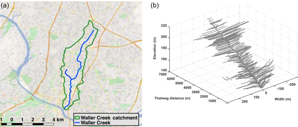
[image:6.612.49.287.183.251.2]The Waller Creek study includes two stream reaches and the catchment area illustrated in Fig. 2. The total stream length is 11.6 km, which drains an area of 14.3 km2. The lay-out of Waller Creek is shown in Fig. 2a, and parts of the bathymetry surveyed data from City of Austin are shown in Fig. 2b for clarity. Two different model geometries were con-sidered, which are designated as WCA and WCB. For WCA, the stream is discretized by 373 computational nodes based on separation of the surveyed cross sections. WCA neglects the minor tributary of Waller Creek and includes the full complexity of the surveyed cross sections shown in Fig. 2b. In contrast, WCB includes both tributaries but uses wider computational node separation with only 30 of the 373 sur-veyed cross sections.
-300 -200
Width (m) -100 0 100 200 300 0 1000 2000 3000 4000
Thalweg distance (m) 5000 6000 220
200
180
160
140 7000
Elevation (m)
(a) (b)
[image:7.612.60.537.68.271.2]Figure 2. (a)Waller Creek and catchment in Austin (Texas, USA).(b)Surveyed cross sections of main channel for Waller Creek (Texas). Only 149 of 327 cross sections are shown for clarity. Elevations are relative to mean sea level (data courtesy of the City of Austin).
Table 1.Cross-section geometry test cases.WBandSswrepresent bottom width and sidewall slope, respectively;f represents the focal
length of parabolic shape.
Channel Number of
Test length computational Cross-section Cross-section case (km) nodes shape type shape detail Case 1 3.1 78 Uniform rectangular WB=20 m
Case 2 0.2 6 Uniform trapezoidal WB=1 m;Ssw=0.5
Case 3 0.3 6 Uniform trapezoidal WB=0.1 m;Ssw=1.5
Case 4 5.6 71 Uniform trapezoidal WB=10 m;Ssw=0.5
Case 5 10 167 Uniform quasi-parabolic f =37.8
Case 6 10 1664 Surveyed bathymetry Unsymmetrical cross section Case 7 122 31 Surveyed bathymetry Unsymmetrical cross section
synthetic inflow data set for the headwater inflows. The syn-thetic flow at each headwater stream was computed based on a downstream peak flow rate distributed uniformly across all the headwater reaches. We used the peak flow rate recorded on the main stem of Guadalupe River at Victoria (Texas) on 19 January 2010 by USGS gauge 08176500. As this gauge does not include the San Antonio River flows, we divided the peak flow rate (453 m3s−1) by the total number of headwater streams in the Guadalupe River (815) to get a single inflow value that was applied to each headwater reach (0.55 m3s−1). The same flow rate was used for the 725 headwater reaches of the San Antonio River network. This approach ensures that there is flow in every branch in the river network.
As is often the case in large river networks, comprehen-sive cross-section geometry data were not available for the San Antonio and Guadalupe rivers. Indeed, Hodges (2013) noted data availability and our ability to effectively use
syn-thetic geometry as one of seven fundamental challenges to continental river dynamics modeling.
Because the geometry affects both PTM and SSM solu-tions, we tested four different estimation approaches for syn-thesizing geometry (Cases A, B, C, and D). Case A uses synthetic trapezoidal cross sections using the approach ap-plied in Liu and Hodges (2014) based on Western et al. (1997). In this method, trapezoidal widths (W) are computed from mean annual flows (Qm) from the NHDPlus data set asW=αQ0m.5withα=1.5. For the side slope of the trape-zoidal cross section, an identical sidewall slope (45◦) is used throughout the river network. Case B channels were similar to Case A but included some minor changes to Manning’s
[image:7.612.119.478.350.472.2]Anto-Figure 3.San Antonio and Guadalupe river network from an NHDPlus V2 flowline.
nio and Guadalupe river network along with the at-a-station hydraulic geometry approach (Rhodes, 1977) to find the best trapezoidal cross-section approximation for the drainage area. Using this approach, the bed width (b0) is an exponen-tial function of cumulative drainage area (AD) as
b0=γ AλD, (10)
where b0 is meters, AD is km2, and the coefficients are
γ =12.59 andλ=0.382. The Santibanez (2015) approach provides reasonable values for trapezoidal channel sidewall slopes over most of the basin but fails in many of the first-order streams with small drainage areas (<25 km2) where the computed sidewall slopes are near zero. For simplicity in the present test cases, a uniform value of 45◦ is used for the sidewall slopes throughout the river network. Case D uses channel bathymetry data generated from Zheng (2016), which use a height above nearest drainage (HAND) anal-ysis (Nobre et al., 2011) applied to the National Elevation Dataset (NED) to provide an automated approach for esti-mating trapezoid-based composite cross sections.
4 Results
4.1 Comparison metrics
The overall algorithm efficiency is evaluated by the number of Newton iterations required for convergence to steady state. The number of Newton iterations reflects the difficulty in converging the nonlinear solution and is proportional to the simulation runtime. As this metric is independent of com-puter architecture, it provides a universal measure of algo-rithm performance. For SSM, we use the number of iterations to converge the area(A) solution of Eq. (6), which is the dominant computational cost (i.e., the non-iterative graph-traversal solution for Q is negligible in comparison). For PTM, we use the cumulative sum of Newton iterations for the(Q, A)solution over all pseudo time steps. Where con-verged solutions of PTM and SSM both exist, comparisons (not shown) indicate the resulting(Q, A)steady-state results are identical within the convergence tolerance (=10−6). 4.2 Effects of cross-section geometry
[image:8.612.99.495.66.365.2]Table 2. Newton iterations required to achieve convergence for benchmark geometry test cases. The converged results are identi-cal for both methods.
Relative Test PTM SSM speed-up case iterations iterations of SSM Case 1 327 6 54×
Case 2 73 4 18×
Case 3 136 8 17×
Case 4 773 9 85×
Case 5 8634 76 113×
Case 6 13 765 4 3441×
Case 7 91 234 30 3041×
appears somewhat erratic, which is likely because the overall number of pseudo time steps depends on how far the starting guess is from the converged answer and the size of the time step used in the PTM pseudo time march.
By comparing the geometric data from Table 1 with the results in Table 2, it can be seen that the largest discrepan-cies between PTM and SSM performance (Cases 6, 7) are with non-uniform cross sections. In both of these, the SSM performsO(103)times better, compared toO(10)toO(102)
improvements for simple geometry cases. This result is con-sistent with the idea that the performance of PTM depends on how close the starting guess for {Q, A}is to the steady-state solution. With non-uniform cross-section geometry, the starting guess is generally quite far from the steady-state con-dition, as it is difficult to a priori estimate gradients of the water surface that match the nonlinear acceleration associ-ated with cross-section variability. In contrast, the benchmark tests with simple cross-section geometry (Cases 1–5) show more modest speed-up by SSM, which is consistent with the steady-state solution for PTM with simple geometry being closer to the starting guess. For short reaches with simple ge-ometry and only a few computational nodes (Cases 2, 3), the speed-up by SSM is essentially irrelevant.
4.3 Scalability
Computing initial conditions using models with varying numbers of computational nodes for Case 4 in Table 1 pro-vides the speed-up results shown in Fig. 4. These tests use simple trapezoidal cross sections and, consistent with the re-sults above, the speed-up advantage of the SSM is relatively modest with less than 103nodes. However, beyond this point, the effective speed-up with SSM is quite dramatic. It appears that the SSM method becomes more effective than PTM both with increasing complexity of the cross-sectional geometry and the increasing number of computational nodes.
Number of computational nodes
102 104 106 108
SSM speed-up multiplier
0 1000 2000 3000 4000 5000 6000
[image:9.612.83.253.105.228.2]SSM speed-up
Figure 4.Speed-up multiplier of SSM compared to PTM for Case 4 as a function of the number of computational nodes.
4.4 Waller Creek test cases
The results of initial condition convergence for two Waller Creek simulations are shown in Table 3. The SSM method dramatically reduces the total number of iterations to con-vergence, which is also reflected in reducing the computer runtime by 99 and 92 % for WCA and WCB, respectively. Although the absolute runtime for this small system is triv-ial for either PTM or SSM, the disparity provides insight into the performance that is confirmed with the more complicated river network (discussed below).
4.5 San Antonio and Guadalupe river basins
Table 3.Total Newton’s iterations required to achieve convergence of the Waller Creek test case.
Pseudo time-marching Steady-solution Relative PTM SSM Configuration iterations (PTM) iterations (SSM) speed-up of SSM runtime runtime WCA 2900 23 130× 1.570 s 0.011 s
WCB 890 13 70× 0.037 s 0.003 s
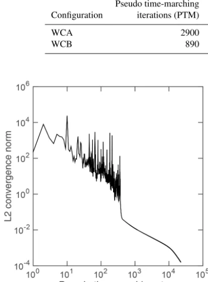
Figure 5.Convergence of the L2 norm between consecutive pseudo time-marching solutions for the PTM with configurationB of the San Antonio and Guadalupe river network. Note the above figure uses the number of time-marching steps as compared to the larger number of Newton iterations provided in Table 4.
successfully converge is not included in the comparisons of Table 4.
The convergence behavior of the PTM for configuration B is shown in Fig. 5. It can be seen that for several hundred time-marching steps the solution was oscillating rather dra-matically but eventually settled down to a slow, smooth be-havior. We believe this is evidence of the PTM trying to overcome inconsistencies between the {Q(t0), A(t0)} start-ing conditions and the boundary conditions in the network. Note that PTM for B was not converged to the same=10−6 tolerance used for SSM. Instead, the solution was manually terminated after more than 9 h, when the convergence norm reached 1.6×10⁻⁴and was sufficiently smooth so that it was clear that the method would eventually converge.
5 Discussion
5.1 Effects on spin-up
As alluded to in the introduction, obtaining an effective model initial condition is only one step in the initialization
of an unsteady model. A second step is understanding at what time the model results are independent of any errors or inconsistencies in the initial conditions – i.e., the spin-up time. Some model spin-up time is generally unavoidable as we never have exactly the correct spatially distributed ini-tial conditions that are exactly consistent with spaini-tially dis-tributed boundary conditions. In effect, eliminating spin-up time requires a set of initial conditions that are not only con-sistent with the boundary conditions att=0 but also con-sistent with the boundary conditions fortm< t <0, where
tmrepresents the system “memory” (or the time interval to wash out a transient impulse).
As an illustration of the scale of the spin-up problem compared to the initial condition problem, we have run the SPRNT unsteady SVE model (Liu and Hodges, 2014) for the San Antonio and Guadalupe river network using over 30 000 data points of unsteady lateral inflows for 14 days in January 2010. These boundary condition data were gener-ated from the North American Land Data Assimilation Sys-tem (NLDAS). The initial conditions were generated using SSM, as described above. The initial conditions were then perturbed by ±20 % in every first-order reach, which pro-vides two slightly different initial condition data sets to com-pare to the baseline. In Fig. 6, the time-marching results for the perturbed and baseline initial condition cases reach the same state throughout the network (0.001 % threshold value) at 152 and 154 h of simulation time, respectively. Thus, ap-proximately 160 h represents a conservative estimate of the expected time for errors in first-order streams to be diluted in the higher-order (larger) river branches. Note that it only takes 3.8 s of CPU time to compute initial conditions using SSM and an additional 5 min of CPU time to compute the time marching during the spin-up interval with the SPRNT unsteady model. This is 2 orders of magnitude faster than the 9 h or more of CPU time required just to compute initial conditions using PTM for the same system.
5.2 Model performance
[image:10.612.66.272.93.372.2]Table 4.Total Newton’s iterations required to achieve convergence for four configurations of the San Antonio and Guadalupe river network.
PTM Newton SSM Newton Relative PTM SSM Configuration iterations iterations speed-up of SSM runtime∗ runtime A convergence failure 61 – – 3 s B 192 527 51 >3775× 9 h 5 min 8 s 3 s C convergence failure 29 – – 6 s D convergence failure 46 – – 14 s
∗The PTM method was terminated after the L2 convergence norm reached 1.6×10⁻⁴, whereas the SSM was converged to the
predefined tolerance of 10−6.
Time (h)
0 50 100 150 200 250 300
Wetted
area
(m
2)
718 720 722 724 726 728
730 Negative 20 % perturbation
No perturbation Positive 20 % perturbation
Figure 6.Spin-up for the San Antonio and Guadalupe river network with the SPRNT unsteady SVE model initialized using the SSM approach. The positive and negative 20 % perturbations are for the
Qinitial conditions in first-order reaches.
systems requires a frustrating trial and error approach to tun-ing the system to obtain convergence. In contrast, the SSM provides a rapid solution to the initial condition problem because Q is computed from simple graph traversal (once through the network), and the subsequent computation ofA
is “local” (in the sense there is no coupling between distant computational nodes). Note that in contrast to PTM, the SSM does not require the modeler to select a set of starting con-ditions; i.e., the SSM starting condition (Q) is defined solely by the t=0 boundary conditions. Thus, different modelers will produce exactly the sameQ(0)andA(0)with the same number of iterations when using the SSM on identical ge-ometry and boundary conditions. This same cannot be said for PTM as modelers must select their{Q(t0), A(t0)} start-ing condition and may need to resort to custom model tunstart-ing to obtain convergence.
Herein, we only tested two methods for initial conditions, both based on finding the steady-state{Q, A}that are consis-tent with the boundary conditions. However, we can also ar-gue that the cold start and synoptic start (see Sect. 1.3) would likely perform as bad or worse than PTM. That the cold start
would perform poorly follows from the fact that it has the ex-act same problem as the PTM (converging over time from in-consistent starting data) but increases the difficulty by trying to converge to the unsteady boundary conditions. A cold start effectively turns the initial condition problem into a spin-up problem. For a cold start model performing similarly to the PTM for the San Antonio and Guadalupe river network, we can expect spin-up to require more than 104time steps of the unsteady solver.
Although it is possible that a synoptic start could per-form better than PTM or a cold start, it seems likely that any approach to interpolating/extrapolating sparse observational data across a larger river network will necessarily result in inconsistencies between the initial{Q, A}and the boundary conditions. If such inconsistencies result in model instabil-ities (a difficult thing to predict), the overall model spin-up time could be extensive. The key problem for the synop-tic start is that it requires judgment as to how to best in-terpolate/extrapolate observational data for initial conditions, which is contrasted to the SSM approach of simply using the actualQ(0)boundary conditions and the steady solver with-out any further choices by the modeler.
Note that the poor performance of the PTM cannot be at-tributed to inefficiencies in the unsteady solver. As discussed in Sect. 5.1, the unsteady solver computed 150 h of unsteady simulation from the SSM about 5 or 1800×faster than real time. This implies that the unsteady solver computed 114 min of real-world unsteady flows in the 3.8 s required for the SSM to compute the steady-state initial condition. Thus, the SPRNT unsteady solver is quite efficient – except when given an inconsistent set of initial and boundary conditions as in the PTM solution.
5.3 Limitations
[image:11.612.54.280.209.389.2]lit-erature (e.g., Cormen et al., 2001) and could be readily ex-tended to the SSM.
Fundamental to the SSM approach is the presumption that there are no places of net flow accumulation or loss through-out the network. All reservoirs and hydraulic structures are treated as pass through so that all the upstream flow is propa-gated through the downstream reaches. However, if there are known locations of accumulation or loss, the river network could be divided into subnetworks with separate SSM solu-tions. For example, upstream of a reservoir an SSM solution can be used to obtain the inflow to the reservoir, which can be used with operating information from the reservoir to provide the correct outflowQfor use in the SSM solution for down-stream reaches. Hydraulic structures that affecth(or dh/dx) as a function ofQcan be readily included in the SSM. To do so merely requires changing the momentum equation in a reach to model the physics of the structure (as is similarly done in unsteady SVE models).
6 Conclusions
It is demonstrated that inconsistencies between initial con-ditions and boundary concon-ditions for a large river network solver of the Saint-Venant equations can lead to long spin-up times or solution divergence. We note that synthetic initial conditions are preferred over observed synoptic initial con-ditions due to the ability of the former to provide smooth and consistent spin-up. Two methods to compute synthetic initial conditions for flow (Q) and cross-sectional area (A) for an unsteady Saint-Venant river network model have been presented. Both approaches use the steady-state solution for
t=0, which provides initial conditions that are smooth and globally consistent with the boundary conditions for the model start time. The PTM is likely similar to undocumented approaches previously used; i.e., application of an unsteady model with constant boundary conditions to achieve a steady solution consistent with initial land surface inflows. For large river networks, the PTM method is slow and inconsistent, arguably depending on the quality of the first guesses for
Q andA and the size of the time step required for a sta-ble pseudo time march. A new SSM is developed to address these issues. The SSM computes the initial conditionQin each reach from the inflow boundary conditions of the en-tire network att=0 by applying a mass-conservative graph traversal technique. The initial conditionAin each reach is found from the solution of the steady-state 1-D momentum equation with known Q. The first-guess problem for A is solved as a normal-flow problem with the Chezy–Manning equation and theQfrom graph traversal. Although SSM quires writing an additional numerical solver rather than re-lying on an existing unsteady solver (as used in PTM) our numerical experiments show that SSM is more robust and consistently faster than PTM. The code for both initial con-dition solvers is publicly available at GitHub (Liu, 2014).
Appendix A: Starting conditions
PTM requires starting conditions (or a first guess) of
{Q(t0), A(t0)} for unsteady solution of Eqs. (1) and (2), whereas SSM needs a first guess only for Ain the solution of Eq. (6). As theQsolution by the graph traversal method for Eq. (5) does not require any starting conditions, it fol-lows that for the PTM the best choice forQ(t0)is the same
Qdeveloped by the simple graph traversal approach used for SSM (i.e., Algorithm 2). To obtain starting conditions forA
in SSM orA(t0)in PTM, a reasonable guess is theA asso-ciated with the “normal depth”, denoted Anfor the starting
Q. The normal depth is obtained from the Chezy–Manning equation solved for normal flow conditions, i.e.,
Q= 1
en
AnRh2/3S01/2. (A1)
The hydraulic radius at normal depth requires the area at normal depth and the wetted perimeter at normal depth,
Rh(n)=An/Pn, which implies Chezy–Manning can be writ-ten as
An= e
nQ
S01/2 !3/5
Pn2/5. (A2)
Thus, an initial guess forAcan be computed for knownQ, en, andS0, whereP =P (A)is a known piece-wise continu-ous function based on river bathymetric data. SinceP (A)is a nonlinear function, Eq. (A2) must be solved with a non-linear solution method. A simple bi-section method can be used following Algorithm 4 with the residual functionr(A)
defined as
r(A)= enQ S01/2
!3/5
P (A)2/5−A=0. (A3)
Note that failure to converge for Algorithm 4 is not nec-essarily fatal; unconverged results are likely to be adequate as they are simply the initial guess for iterative solution by PTM or SSM. As a further simplification, it seems likely that theP (A)in Eq. (A2) could be approximated using a simple rectangular cross section,P (A)=W+2A/W, where known channel widths (W) are used. This simplification is valuable in continental-scale river network simulations, where ade-quate river geometric data throughout a network cannot be guaranteed (Hodges, 2013).
Algorithm 4Bi-section method
1: procedureBiSectionQ,n,S0,Nmax,{: tolerance}
2: Au←0.01 {Search for upper bound}
3: repeat
4: Au←2Au
5: Evaluater(A)in Eq. (A3) 6: unitlr >0
7: Al←0
8: for i=1 toNmaxdo {Bisection method}
9: rl←r(Al)
10: ru←r(Au)
11: Am←(Au+Al)/2
12: if |ru−rl|< then
13: return Am
14: else
15: rm←r(Am)
16: if rm>0then
17: Au←Am
18: else
19: Al←Am
20: end if
21: end if
22: end for
23: return Am
24: end procedure
Notation
A Cross-sectional area (m2)
b0 Trapezoidal channel bed width (m)
b1 Trapezoidal channel sidewall slope DA Drainage area (mile2)
g Gravitational acceleration (ms−2)
f Generic function
F Equivalent friction geometry (m−10/3)
h Depth (m)
en Manning’s roughness (m −1/3s)
P Wetted perimeter (m)
Q Volumetric flow rate (m3s−1)
ql Flow rate per unit length through channel sides (m2s−1)
r Residual function
Rh Hydraulic radius (m)
S0 Channel bottom slope
Sf Channel friction slope S Strahler order
t Time (s)
W Channel width (m)
Competing interests. The authors declare that they have no conflict of interest.
Acknowledgements. This material is based upon work supported by the US National Science Foundation under grant no. CCF-1331610. Edited by: Insa Neuweiler
Reviewed by: Rodrigo Cauduro Dias de Paiva and one anonymous referee
References
Abbott, M., Bathurst, J., Cunge, J., O’connell, P., and Rasmussen, J.: An introduction to the European Hydrological System – Systeme Hydrologique Europeen, “SHE”, 2: Structure of a physically-based, distributed modelling system, J. Hydrol., 87, 61–77, 1986.
Ajami, H., McCabe, M. F., Evans, J. P., and Stisen, S.: Assessing the impact of model spin-up on surface water-groundwater interac-tions using an integrated hydrologic model, Water Resour. Res., 50, 2636–2656, https://doi.org/10.1002/2013WR014258, 2014. Beighley, R., Eggert, K., Dunne, T., He, Y., Gummadi, V., and
Verdin, K.: Simulating hydrologic and hydraulic processes throughout the Amazon River Basin, Hydrol. Proc., 23, 1221– 1235, 2009.
Caleffi, V., Valiani, A., and Zanni, A.: Finite volume method for simulating extreme flood events in natural channels, J. Hydraul. Res., 41, 167–177, 2003.
Chau, K. W. and Lee, J. H.: Mathematical modelling of Shing Mun River network, Adv. Water Resour., 14, 106–112, 1991. Cormen, T. H., Leiserson, C. E., Rivest, R. L., and Stein, C.:
Intro-duction to algorithms, MIT press Cambridge, 2, 2001.
Cunge, J.: Evaluation problem of storm water routing mathematical models, Water Res., 8, 1083–1087, https://doi.org/10.1016/0043-1354(74)90152-3, 1974.
Cunge, J. A., Holly, F. M., and Verwey, A.: Practical aspects of com-putational river hydraulics, Pitman Publishing, 1980.
David, C. H., Maidment, D. R., Niu, G.-Y., Yang, Z.-L., Habets, F., and Eijkhout, V.: River Network Routing on the NHDPlus Dataset, J. Hydrometeorol., 12, 913–934, 2011.
de Saint-Venant, A. B.: Thé orie du mouvement non permanent des eaux, avec application aux crues des rivié res et à l’introduction des maré es dans leurs lits, Comptes Rendus des séances de l’Académie des Sciences, 73, 237–240, 1871.
Hodges, B. R.: Challenges in Continental River Dynamics, Environ. Model. Soft., 50, 16–20, 2013.
Hodges, B. R. and Liu, F.: Rivers and electrical networks: Crossing disciplines in modeling and simulation, Founda-tions and Trends in Electronic Design Automation, 8, 1–116, https://doi.org/10.1561/1000000033, 2014.
Kazolea, M. and Delis, A.: A well-balanced shock-capturing hybrid finite volume–finite difference numerical scheme for extended 1-D Boussinesq models, Appl. Numer. Math., 67, 167–186, 2013. Kvoˇcka, D., Falconer, R. A., and Bray, M.: Appropriate model use
for predicting elevations and inundation extent for extreme flood events, Nat. Hazards, 79, 1791–1808, 2015.
Lax, P. D.: Gibbs phenomena, J. Sci. Comput., 28, 445–449, 2006. Liang, D., Falconer, R. A., and Lin, B.: Comparison between
TVD-MacCormack and ADI-type solvers of the shallow water equa-tions, Adv. Water Resour., 29, 1833–1845, 2006.
Liu, F.: SPRNT: a river dynamics simulator, https://github.com/ frank-y-liu/SPRNT (last access: 23 December 2016), 2014. Liu, F. and Hodges, B. R.: Applying microprocessor analysis
meth-ods to river network modeling, Environ. Model. Soft., 52, 234– 252, https://doi.org/10.1016/j.envsoft.2013.09.013, 2014. Nobre, A., Cuartas, L., Hodnett, M., Rennó, C.,
Ro-drigues, G., Silveira, A., Waterloo, M., and Saleska, S.: Height Above the Nearest Drainage – a hydrologi-cally relevant new terrain model, J. Hydrol., 404, 13–29, https://doi.org/10.1016/j.jhydrol.2011.03.051, 2011.
Paiva, R. C. D., Collischonn, W., Bonnet, M. P., and de Goncalves, L. G. G.: On the sources of hydrological prediction uncer-tainty in the Amazon, Hydrol. Earth Syst. Sci., 16, 3127–3137, https://doi.org/10.5194/hess-16-3127-2012, 2012.
Ponce, V. M., Simons, D. B., and Li, R.-M.: Applicability of kine-matic and diffusion models, J. Hydraul. Eng. Div-ASC, 104, 353–360, 1978.
Pramanik, N., Panda, R. K., and Sen, D.: One dimensional hydrody-namic modeling of river flow using DEM extracted river cross-sections, Water Resour. Manag., 24, 835–852, 2010.
Preissmann, A.: Propagation des intumescences dans les canaux et rivieres, in: Premier Congres De L’Association Francaise de Cal-cul AFCAL, Grenoble 14–16 1960, Gauthier-Villars, Paris, 433– 442, 1961.
Preissmann, A. and Cunge, J.: Calcul du mascaret sur machine élec-tronique, La Houille Blanche, 16, 588–596, 1961.
Rahman, M. M. and Lu, M.: Model Spin-Up Behavior for Wet and Dry Basins: A Case Study Using the Xinanjiang Model, Water, 7, 4256–4273, 2015.
Rhodes, D. D.: The b-f-m diagram; graphical representation and in-terpretation of at-a-station hydraulic geometry, Am. J. Sci., 277, 73–96, 1977.
Sanders, B. F.: High-resolution and non-oscillatory solution of the St. Venant equations in non-rectangular and non-prismatic chan-nels, J. Hydraul. Res., 39, 321–330, 2001.
Santibanez, A. R. H.: Evaluating river cross section geometry for a hydraulic river routing model: Guadalupe and San Antonio river basins, Master’s thesis, The University of Texas at Austin, the United State, 2015.
Seck, A., Welty, C., and Maxwell, R. M.: Spin-up be-havior and effects of initial conditions for an integrated hydrologic model, Water Resour. Res., 51, 2188–2210, https://doi.org/10.1002/2014WR016371, 2015.
Western, A. W., Finlayson, B. L., McMahon, T. A., and O’Neill, I. C.: A method for characterising longitudinal irregularity in river channels, Geomorphology, 21, 39–51, https://doi.org/10.1016/S0169-555X(97)00023-8, 1997. Yang, L., Hals, J., and Moan, T.: Comparative Study of Bond Graph
Models for Hydraulic Transmission Lines With Transient Flow Dynamics, ASME, J. Dyn. Sys., Meas., Control., 134, 13 pp., https://doi.org/10.1115/1.4005505, 2012.
Zhao, D., Shen, H., Lai, J., and III, G. T.: Approximate Riemann solvers in FVM for 2D hydraulic shock wave modeling, J. Hy-draul. Eng., 122, 692–702, 1996.