Munich Personal RePEc Archive
Longevity hedge effectiveness: a
decomposition
Cairns, Andrew and Dowd, Kevin and Blake, David and
Coughlan, Guy
Pensions Institute
May 2011
Online at
https://mpra.ub.uni-muenchen.de/34236/
DISCUSSION PAPER PI-1106
Longevity Hedge Effectiveness: A
Decomposition
Andrew J.G. Cairns, Kevin Dowd, David Blake, and
Guy D. Coughlan
May 2011
ISSN 1367-580X
The Pensions Institute
Cass Business School
City University London
106 Bunhill Row
London EC1Y 8TZ
UNITED KINGDOM
Longevity Hedge Effectiveness: A Decomposition
Andrew J.G. Cairns, Kevin Dowd, David Blake, and Guy D. Coughlan1
First version: September 2010 This version: May 27, 2011
Abstract
We use a case study of a pension plan wishing to hedge the longevity risk in its pension liabilities at a future date. The plan has the choice of using either a cus-tomised hedge or an index hedge, with the degree of hedge effectiveness being closely related to the correlation between the value of the hedge and the value of the pen-sion liability. The key contribution of this paper is to show how correlation and, therefore, hedge effectiveness can be broken down into contributions from a number of distinct types of risk factor. Our decomposition of the correlation indicates that population basis risk has a significant influence on the correlation. But recalibration risk as well as the length of the recalibration window are also important, as is cohort effect uncertainty. Having accounted for recalibration risk, parameter uncertainty and Poisson risk have only a marginal impact on hedge effectiveness.
Our case study shows that longevity risk can be substantially hedged using index hedges as an alternative to customised longevity hedges and that, as a consequence, index longevity hedges – in conjunction with the other components of an ALM strategy – can provide an effective and lower cost alternative to both a full buy-out of pension liabilities or even to a strategy using customised longevity hedges.
Keywords: hedge effectiveness, correlation, mark-to-model, valuation model, sim-ulation, value hedging, longevity risk, stochastic mortality, population basis risk, recalibration risk.
1
Introduction
Hedging the longevity risk in pension plans – the risk that, in aggregate, plan mem-bers live longer than anticipated – is becoming increasingly important. As more defined benefit pension plans close to future accrual and pension liabilities accord-ingly become crystallised, plan sponsors face the choice of selling their legacy pension liabilities or retaining them on their books and managing them.
The UK was the first country in the world to witness the development of both a buy-out market for pension liabilities and a longevity swap market to help sponsors
hedge longevity risk as part of an asset-liability management (ALM) strategy.
With a buy-out, an insurance company, in exchange for a buy-out fee, takes over the plan liabilities and assets and takes on the responsibility for making the pension payments until the last plan member dies. A buy-out is known as an insurance indemnification solution, since all risks in the pension plan – the key ones being interest-rate, inflation-rate and longevity risk – are fully transferred from the sponsor to the insurer. The cost of a buy-out is high since the insurer has to post substantial regulatory capital to ensure that the pension payments will be made with a high degree of probability, as well as to ensure, ex ante, that the purchase price offers an adequate expected return relative to the risks being transferred. In addition to transferring all the pension assets, the sponsor might also need to make a cash payment to the insurer if the plan is in deficit, in order to fund the buy-out. Further, the sponsor foregoes the opportunity to manage the pension assets efficiently itself and so reduce the ultimate cost of the liability.
In contrast, a sponsor might decide to retain the pension plan and implement an ALM strategy, which broadly replicates the same economic effect as a buyout. This brings certain cost advantages. First, the sponsor saves making the buyout risk premium which would otherwise be paid to the insurer as compensation for taking on the risks associated with the pension plan. Second, the cost of each compo-nent of the ALM strategy can be separately negotiated and implemented, providing greater transparency, minimal upfront hedging costs (since the principal hedging instruments are interest-rate, inflation-rate and longevity swaps) and flexibility in the timing and structure of implementation. However, the key disadvantage of such an ALM strategy – which has been dubbed a “do-it-yourself” (DIY) buy-out – is that the risks are not perfectly hedged. This is due to the idiosyncracies of each pension plan’s membership and benefit structure. Swaps can hedge a significant proportion of the relevant risks in a given pension plan, but inevitably there will be some residual basis risk which cannot be hedged cost-effectively using capital market instruments.
Plan sponsors therefore face two key trade-offs. One is between the high costs and complete indemnification of a buy-out versus the lower costs and basis risk associated with a DIY-buyout/ALM strategy. The other, within the context of ALM, is between the higher costs and minimal basis risk of a customised longevity swap versus the lower costs and greater liquidity but higher basis risk associated with an index swap.
1.1
Analysis and evaluation of longevity hedges
In this paper, we examine we examine the trade-off between customised and index longevity hedges. Coughlan et al. (2011) proposed a clear framework for “(i) de-veloping an informed understanding of the basis risk, (ii) appropriately calibrating the hedging instrument and (iii) evaluating hedge effectiveness”. In this paper, we follow closely Coughlan et al. (2011) both in terms of the framework and the first of their case studies. However, the key difference, and the main contribution, in the present work is that whereas Coughlan et al. used a largely model-free bootstrap-ping approach to the evaluation of hedge effectiveness in their case study, we use a model-based simulation approach in our study. As will be demonstrated later, this allows us to break down basis risk and the evaluation of hedge effectiveness into a number of components by switching on and off a number of key risk factors.
Our case study involves the use of England & Wales male mortality (the LifeMetrics index) to hedge liabilities linked to Continuous Mortality Investigation (CMI) male assured lives mortality. The case study considers a value hedge (as opposed to a cashflow hedge) set up at time 0 of a pension plan liability’s exposure to longevity risk at a single future valuation date, T.2 The hedging instrument that we use will
be a “cash-settled” deferred longevity swap, (defined later). Decomposing the corre-lation between the hedging instrument and the liability values is broadly equivalent to decomposing theeffectiveness of the hedge.
There are three key categories of factor that contribute to an assessment of hedge effectiveness or the correlation between a hedging instrument and the liability being hedged:
1. Factors related to population differences, including:
• Population basis risk: this arises as a result of using a hedging instru-ment linked to a different reference population from that of the hedging population.
• Mismatched cohorts especially at younger ages: typically, the hedger of population 2 will wish to hedge the longevity risk for an existing group of plan members with accrued pension rights: that is, there will be some historical data for that cohort. However, the hedger might choose to link their hedging instrument to a cohort born in a different year (resulting in an age mismatch). In theory, this reference cohort might be one for which there will be no data until after time 0. In this case, the value of the hedging instrument at T has the cohort effect as an additional source of uncertainty that will have a deterimental impact on hedge effectiveness.3
2. Factors related to the model used for simulation, including:
• The choice of model to be fitted to historical mortality data and how the parameters and latent state variables of this model will be calibrated. This model will be used to simulate future mortality scenarios which will then, one by one, be fed into the valuation model discussed below.4
• Parameter uncertainty: arises because the true values of the parame-ters of the simulation model used to generate future mortality scenarios and quantify longevity risk are unknown – this covers both the process parameters (i.e., parameters governing the dynamics of the underlying stochastic processes) and the latent state variables of the model (i.e., the underlying age, period and cohort effects).
• Poisson risk:5 otherwise known as small-population risk or sampling
vari-ation; the risk that the mortality experience of a small group of people will differ from the underlying true mortality rate; the financial consequences can be magnified if there is significant variation between individuals in pension entitlements.6
3. Factors related to the model used for valuation at the future valuation date,
T:
• The choice of model to be used to value liabilities at timeT. This model is likely to be different from the simulation model.7
3This means that, in practice, linkage to a future cohort would be suboptimal and not to be recommended.
4There is model risk associated with the simulation model, since we do not know the true model generating future mortality rates: we disregard this risk in this study.
5So-called because deaths in the pension plan are assumed to follow a Poisson distribution; see, e.g., Dahl et al. (2008) and Li and Hardy (2009), and see, e.g., Li et al. (2009) for alternative assumptions.
6We do not consider this so-called ‘big cheese’ risk explicitly in the present paper.
• Recalibration risk: the uncertainty in both future liability values and hedging-instrument values associated with the calibration and recalibra-tion of the parameters of the valuarecalibra-tion model used to project mortality beyond the measurement date. The valuation model contains a num-ber of process parameters that are assumed to be remain constant over time. However, the model will normally be calibrated using the latest available data. Thus, the calibration will be dependent on the specific scenario under consideration, and will be based solely on observed deaths and exposures rather than assuming knowledge of the underlying latent state variables. The extent to which valuation model parameters vary from one simulation sccenario to the next results in additional random-ness in liability and hedging-instrument values at T. Recalibration risk is, therefore, heavily dependent on the scenarios generated by the sim-ulation model and includes the influence of both parameter uncertainty and Poisson risk.
• Recalibration window: the length of the lookback window over which the valuation model is estimated and subsequently recalibrated; this reflects a tradeoff between using more years of data to get a better estimate of the volatility in the data and using fewer years of data to get a better estimate of the current trend in mortality improvements; it has a direct influence on recalibration risk.
4. Factors related to the structure of the hedge, such as:
• Choice of hedging instrument.
• Choice of maturity date, reference population and reference age(s).
• Sub-optimal or inaccurate hedge ratio.
• Robustness of the hedge ratio: the challenge is to devise strategies that can maximise hedge effectiveness and to find solutions that are robust relative to, for example, errors in the specification of the model and pa-rameters, etc.
• Index versus customised hedges.
• Static versus dynamic hedges.8
• Multi-instrument9 versus single-instrument hedges.
The above list is quite extensive and it would not be feasible to examine all pos-sible factors in a single study. Nevertheless, ours is the first study to carry out a forensic analysis of what we anticipate being the most important risk factors in a longevity hedging context, namely population basis risk, cohort effect uncertainty,
8In this paper, we only consider static hedges (i.e. “set and forget”). However, especially if there was a liquid market in appropriate hedging instruments, the hedge ratios could be modified from time to time between commencement and the target valuation date.
recalibration risk, the impact of the length of the recalibration window, parameter uncertainty, and Poisson risk.
Previous studies which have examined a smaller subset of risk factors include: Dahl et al. (2008, 2009), Plat (2009), and Coughlan et al. (2011). Earlier studies which have examined different hedging instruments, such as longevity swaps, deferred longevity swaps and other longevity-linked bond and derivative structures, include Blake and Burrows (2001), Blake et al. (2006), Coughlan et al. (2007), Loeys et al. (2007), Cairns et al. (2008), Coughlan (2009), Wills and Sherris (2010), and Blake et al. (2010). Previous studies which have looked at the value-hedging paradigm include Coughlan et al. (2011) – in terms of effective risk reduction when future cashflows are highly unpredictable – and Nielsen (2010) and Olivieri and Pitacco (2009) in the context of Solvency II.
We find in this paper that recalibration risk has an important role to play in the assessment of hedge effectiveness. This is because we have a limited amount of historical data, leading to parameter uncertainty in both process parameters and the underlying state variables. This paper is the first to consider recalibration risk in the longevity literature. However, the concept is familiar elsewhere in the finance literature. The key issue is that model parameters that are assumed to remain constant are, in fact, recalibrated on a regular basis: partly because of parameter uncertainty and partly because the “true” model generating prices is different from the model being calibrated against these prices (e.g. the Black-Scholes model). The result is a sequence of calibrations that is inconsistent with the constant-parameter assumption. The fact that, for example, equity volatility is known to vary over time (as well as over strike prices and maturity dates) rather than remain constant, results in derivatives desks having to hedge against changes in volatility (vega hedging).
A related, but different, form of calibration risk concerns the method use to calibrate a complex model to a given set of market data (see, for example, Detlefsen and H¨ardle, 2007). The nearest equivalent in the mortality modelling context would, perhaps, be the choice between the Poisson model for death counts and some other distribution (e.g. the normal distribution assumed by Lee and Carter, 1992).
We also find that the major determinants of correlation, and therefore hedge ef-fectiveness, are population basis risk and the length of the recalibration window. Lesser, but still important factors are: parameter uncertainty (other than recalibra-tion risk) and the reference age for the hedging instrument (especially if the reference age is at the lower end of the age range analysed).
1.2
Structure of the paper
and discusses the role of correlation (between the values of the hedging instrument and the liability) in determining the level of hedge effectiveness. Section 4 describes the data and stochastic mortality model that we will use. Section 5 discusses how the model is used for both (i) simulating future mortality rates and (ii) valuing both the liability (a type of deferred annuity) and the hedging instrument. Although the choice of simulation model is independent of the choice of valuation model and is borne out in industry practice, we use the same model for convenience. Section 6 is the key numerical section that focuses on the correlation between the value of the pension liability in our case study and the values of both customised and index-based hedging instruments and quantifies how the different risk factors influence these correlations. Finally, Section 7 concludes.
2
A case study: A customised versus index hedge
Our discussion is centred on a stylised case study involving a UK pension plan consisting of male members only, which pays no spouses’ or dependants’ benefits. We evaluate hedging instruments that hedge the longevity risk associated with the value of the pension liability. The pension plan members will be assumed to have underlying mortality rates that are the same as the CMI male assured lives dataset and the pension liability will be calculated with reference to current and projected CMI mortality. This choice is because the CMI population has a very different mortality profile from the national population (see for example, Coughlan et al., 2011), thereby allowing us to easily incorporate the population basis risk into the discussion. In order to hedge the longevity risk in the pension plan, we will consider both a hedging instrument linked to CMI male mortality (in the case of a customised hedge) and one linked to England & Wales (EW) male mortality (in the case of an index hedge). Data are available for both populations up to the end of 2005 (time
t= 0).
Now define ak(T, x) as the value at T of a pension (or, equivalently, a life annuity)
of£1 per annum payable annually in arrears from the time of retirement until death
to a male aged x at timeT in populationk:
k = 1 England & Wales, males
k = 2 CMI assured lives, males.
The objective is to hedge the longevity risk in the value of a pension liabilityL(T) =
a2(T, x), whereT = 10 years (i.e., the end of 2015) andx= 65. We assume that the
pension is already in payment: i.e. the members have already reached the age of retirement. Interest rates will be assumed to be constant and equal torper annum. Hence, the liability at time T is equal to
ak(T, x) =
∞
X
s=1
(1 +r)−s
where the forward (prospective) survival probability, pf wdk (T, s, x), represents the best estimate at T, that an individual agedx at timeT in population k will survive for a furthers years.
In our case study, the chosen hedging instrument will be a “cash-settled” deferred longevity swap that exchanges, at time T, the present value of a series of fixed cashflows for the present value of a set of floating cashflows occurring after time
T. The floating cashflows will be equal to the proportions of a cohort aged y in population k at time T that are still alive at times T + 1, T + 2, . . ., while the fixed cashflows of K(T +s) for s = 1,2, . . . are fixed at time 0. Thus, the value at time
T of the floating leg of the swap will be ak(T, y) (i.e., the same as the value of an
annuity) and we will denote the value atT of the fixed leg by ˆaf xdk (T, y).
3
Constructing and evaluating a hedge
3.1
The hedge effectiveness framework
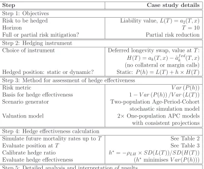
Following the proven framework of Coughlan et al. (2004, 2011), there are five steps in constructing and evaluating a hedge – whether customised or index. These steps have been slightly recast in applying them to our case study and are outlined in Tables 1 to 3.
Step 1 in Table 1 involves a clear definition of the hedging objectives. This includes defining the position to be hedged and the hedge horizon, T. In our case study, the metric, or quantity at risk, to be hedged is the value of the liability,a2(10,65), over
a horizon of 10 years. This step also involves a clear definition of the risk to be hedged and whether to mitigate it entirely (indemnification) or whether to mitigate it partially (leaving some degree or other of residual basis risk).
In step 2, we choose the hedging instrument, or instruments, that we will use to reduce the liability risk. In the present case, it will be a deferred longevity swap, with a choice of reference population,k,10 maturity dates,T, and reference starting
ages, y. The hedge will be a static value hedge.11
Step 3 is the crucial step of defining the method for hedge effectiveness assessment. This is important because an inappropriate choice can easily lead to misleading hedge effectiveness results. This step involves not only the risk metric used to assess hedge effectiveness but also the method in which it is applied. For our case study, we choose the variance in the value of the pension liability as the risk measure (the same as, for example, Li and Hardy, 2009). Hedge effectiveness then provides us with a proportionate assessment of how much the variance of the liabilty will fall as a result of hedging.
10k= 1 for an index swap andk= 2 for a customised swap.
Step Case study details
Step 1: Objectives
Risk to be hedged Liability value, L(T) =a2(T, x)
Horizon T = 10
Full or partial risk mitigation? Partial risk reduction Step 2: Hedging instrument
Choice of instrument Deferred longevity swap, value at T:
H(T) = ak(T, x)−ˆaf xdk (T, x)
(no collateral or margin calls) Hedged position: static or dynamic? Static: P(h) = L(T) +h×H(T) Step 3: Method for assessment of hedge effectiveness
Risk metric V ar(P(h))
Basis for hedge effectiveness 1−V ar(P(h))/V ar(L(T)) Scenario generator Two-population Age-Period-Cohort stochastic simulation model Valuation model 2× One-population APC models with consistent projections Step 4: Hedge effectiveness calculation
Simulate future mortality rates up toT See Table 2 Evaluate position at T See Table 3 Calibrate hedge ratio h∗
=−ρLH ×SD(L(T))/SD(H(T))
Evaluate hedge effectiveness (h∗
[image:11.595.84.499.94.439.2]minimises V ar(P(h))) Step 5: Detailed analysis and interpretation of results
Table 1: Five steps in constructing and evaluating a hedge (adapted from Coughlan et al., 2011).
We take a prospective approach to hedge effectiveness assessment using forward looking simulation of future mortality rates (see Coughlan et al., 2004, for a discus-sion of this and other choices). The risk measure is derived from a large number of independent scenarios for mortality rates between time t = 0 and time T that are generated using a stochastic simulation model.12
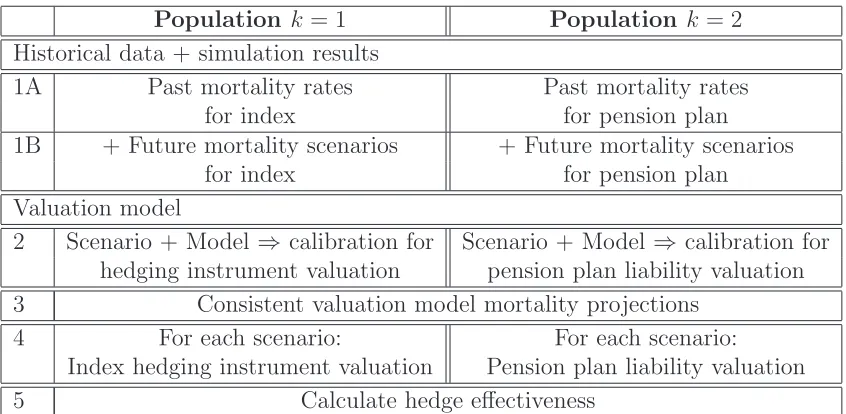
There are two key stages in Step 4: simulation and valuation. First, there is a simulation stage that takes us from the present time t = 0 to time T (see Table 2). This requires a two-population stochastic mortality model13 to be calibrated to
historical data up to time t = 0 that can then be used to simulate future mortality rates for both populations to time T. Second, for each stochastic scenario up to timeT, we need to be able to value the liability and hedging instrument at time T. Valuation of these requires us to project, atT, the future liability cash flows beyond time T (see Table 3). We, therefore, extend each sample path of mortality rates up
12There are other methods of generating these scenarios, for example, Coughlan et al. (2011) used bootstrapping of historical data.
Population k = 1 Population k = 2 1 Past mortality rates Past mortality rates
for index population for pension plan (up to time “t= 0”) (up to time “t = 0”) 2 Fit two-population model
3 Simulation of two-population underlying mortality rates for t = 1, . . . , T
4 Index population: Add Pension plan: Add Poisson risk to death counts Poisson risk to death counts 5 Future scenarios for index Future scenarios for pension plan
[image:12.595.83.472.151.322.2]mortality experience, t = 1, . . . , T mortality experience, t= 1, . . . , T
Table 2: Five stages of simulation
Population k = 1 Population k= 2
Historical data + simulation results
1A Past mortality rates Past mortality rates for index for pension plan 1B + Future mortality scenarios + Future mortality scenarios
for index for pension plan Valuation model
2 Scenario + Model⇒ calibration for Scenario + Model ⇒ calibration for hedging instrument valuation pension plan liability valuation 3 Consistent valuation model mortality projections
4 For each scenario: For each scenario:
Index hedging instrument valuation Pension plan liability valuation 5 Calculate hedge effectiveness
[image:12.595.82.505.464.671.2]to timeT into a two-dimensional mortality table that projects beyond timeT. The final year of the simulated scenario at time T gives us the base, one-dimensional mortality table, and the pattern of mortality improvements up to time T are used to turn this base mortality table into a two-dimensional set of projected mortality and survival rates that can be used to calculate annuity values at T. We are then in a position to evaluate hedge effectiveness.
In other words, the outcome from the simulation and valuation procedures is a bivariate distribution for the liability and hedging instrument values atT. This, in combination with our chosen measure of hedge effectiveness, allows us to calculate the optimal hedge ratio, h∗
.
Step 5 analyses the results of steps 1 to 4. This includes testing the robustness of our solutions to the assumptions used in the calculations, as well as assessing whether the results make intuitive sense.
3.2
Correlation and hedge effectiveness
Ultimately, our aim is to measure the effectiveness of any hedging strategy that we might choose to adopt. Here we focus on a simple value-hedging setting where we consider a static (set-and-forget) hedge using a single hedging instrument.
Suppose that we have a future random liability with value L = L(T) at time T. Alongside this, we have a hedging instrument that has valueH =H(T) at time T. Our hedged portfolio consists of the liability plushunits (the hedge ratio) ofH and its value at T isP(h) =L+h.H.
If we use variance as our measure of risk, hedge effectiveness is defined as R2(h) =
1−V ar[P(h)]/V ar[L]: that is, it measures the proportionate reduction in risk due to the hedge. The optimal hedge ratio per unit of liability, L, then becomes
h∗
=−ρSD(L) SD(H) =−
Cov(L, H)
V ar(H) ,
whereρ=Cor(L, H) (see, for example, Coughlan et al., 2004, for a general discus-sion of the optimal hedge ratio in a hedge effectiveness context). We then have
R2(h∗
) =ρ2 and R2(h) = ρ2
µ
1− (h−h
∗ )2
h∗2
. (2)
We can conclude from (2) that, in this simple situation with a static hedge and a single hedging instrument, it is sufficient for us to analyse the correlation between
4
Data and model
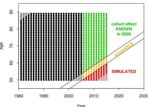
We will use EW and CMI data covering ages 50 to 89 and calendar years 1961 to 2005 (with 2005 treated ast= 0). The full range of these data is used to fit the two-population stochastic mortality model specified below. This model plus parameter estimates – with some, but not all, experiments incorporating parameter uncertainty – is then used to simulate mortality rates at ages 50 to 89 for the years 2006 to 2015. The choice of age range means that the CMI cohort aged 65 in 2015 – the cohort that we refer to in our liabilityL(T) =a2(T,65) – was aged 55 in 2005. Thus, our
initial dataset up to 2005 already provides us with an estimate of the cohort effect that will be used in the evaluation of a2(T,65).
For valuation purposes, actuaries will be deemed to have data available from 1961 up to the end of 2015. However, a projection model intended to project beyond time
T will only be calibrated using data from the most recent 20 years (1995 to 2015) in order to capture the most recent trend in mortality rates. The assumption of a 20-year lookback window is consistent with market practice (not all practitioners, of course, will use exactly 20 years), whereby the desire to use more years of data to get a better estimate of the volatility needs to be balanced by the desire to use fewer years in order to capture better the most recent trend in mortality improvements (see the discussion in Dowd et al., 2010b).14
We will use the two-population Age-Period-Cohort (APC) model for mk(t, x), the
population-kdeath rate, discussed in Cairns et al. (2011b).15 Specifically, we assume
that
logmk(t, x) = β(k)(x) +
1
na
κ(k)(t) + 1
na
γ(k)(t−x) (3)
where: tis the calendar year;xis the age last birthday;nais the number of individual
ages covered by the dataset;16 β(1)(x) and β(2)(x) are the population 1 and 2 age
effects, respectively; κ(1)(t) and κ(2)(t) are the corresponding period effects; γ(1)(c)
and γ(2)(c) are the corresponding cohort effects; and c = t− x = cohort year of
birth.
This model is one of the simplest that incorporates both random period and cohort effects. Our reasons for including a cohort effect are twofold. First, cohort effects have been found to be significant in a number of countries (e.g. England & Wales, France, Germany, Japan and Italy; see Cairns et al., 2011a). Second, when we consider possible hedges of longevity risk, we build on the observations of Cairns et al. (2011b) to demonstrate that the presence of a significant cohort effect can have a material impact on correlation and, implicitly, hedge effectiveness in a way that
14However, even if our use of the APC model for valuation is correct, the use of a 20-year window,
W, should itself be considered to be a source of Knightian uncertainty: W is not just uncertain, but the degree of uncertainty is not quantifiable. Dealing withW as a source of uncertainty is left for further work.
15Alternative multi-population models have been proposed by Li and Lee (2005), Dahl et al. (2008, 2009), Jarner and Kryger (2011), Plat (2009) and Dowd et al. (2011a).
16For example, our dataset covers ages 50 to 89, son
would not be evident if a model with no stochastic cohort effect were used.
The stochastic elements in our model (i.e., the period and cohort effects) are struc-tured in a way that assumes that one population is large and the other population is a small (sub-)population. Thus (see Cairns et al., 2011b, for further discussion),
• Large population 1
– κ(1)(t) is modelled as a random walk with drift µ 1.
– γ(1)(c) is modelled as an AR(2) process mean-reverting to a linear trend.
(This has the ARIMA(1,1,0) model as a special limiting case.)
• The smaller population 2 is modelled indirectly using the spreads in the period and cohort effects:
– The spread between period effects, S2(t) = κ(1)(t)−κ(2)(t), is modelled
as an AR(1) process with, potentially, a non-zero mean-reversion level. Random innovations in the AR(1) process are correlated with theκ(1)(t)
innovations.
– The spread between cohort effects, S3(c) = γ(1)(c)−γ(2)(c), is modelled
as an AR(2) process with, potentially, a non-zero mean-reversion level. Random innovations in the AR(2) process are correlated with theγ(1)(c)
innovations.
• Random innovations in the bivariate period-effect processes are assumed to be independent of random innovations in the bivariate cohort-effect processes.
The equations for this model are presented in Appendix A, and for a fuller discussion of the model, see Cairns et al. (2011b). A key element of the model fitting process in Cairns et al. (2011b) is the use of Bayesian methods.17 The approach starts by
combining the statistical likelihood functions for the death counts and the time series of underlying period and cohort effects: especially important where one or both of the populations are relatively small. Additionally, Bayesian methods produce a full posterior distribution both for process parameters (µ1, µ2, ψ, C(2), ν1, δ1, ν2, φ11,
φ12, φ21, φ22, C(3)) and for historical values of the age, period and cohort effects.18
The posterior distribution can then be used in a natural way to analyse the impact of parameter uncertainty on the results of our present analysis.
17For further discussion of mortality model fitting using Bayesian methods, see Czado et al. (2005), Pedroza (2006), Kogure et al. (2009), Reichmuth and Sarferaz (2008), and Kogure and Kurachi (2010).
5
Simulation and valuation
5.1
Simulation
Simulation involves the following stages:
• First, in the case where we assume the parameters are unknown, we draw at random from the posterior distribution for the process parameters and for the historical age, period and cohort effects.
• Next, we use simulation to extend the historical sequences of period and cohort effects by T years using the time series model discussed in Section 4. This then allows us to calculate the underlying death rates, mk(t, x), for years t =
1, . . . , T using equation (3).
• Finally, in experiments where we wish to take individual Poisson risk into account, we need to specify exposures and simulate death counts. Thus, we need to define what the exposures, Ek(t, x), are for t = 1, . . . , T, and then to
simulate numbers of deaths using the Poisson assumption:19 that is,
Dk(t, x)∼Poisson (Ek(t, x).mk(t, x)).
The output from the simulation step is, therefore, a set of deaths and exposures, rather than direct observation of the underlying death rates.
In the analysis that follows, we consider two cases that concern the specification of the exposures for the years 2006 to 2015:
• Case 1 (standard “Poisson risk” case). We set the exposures for 2006 to 2015 to be equal to their 2005 levels: that is, Ek(t, x) = Ek(0, x) for k = 1,2,
t= 1, . . . ,10 and for all x.
• Case 2 (the large population or “no Poisson Risk” case). We set Ek(t, x) =
100×Ek(0, x) for k= 1,2,t= 1, . . . ,10 and for all x.20
In both cases, exposures mostly decline with age from their 2005 values. However, we have not adjusted values to reflect cohorts of varying sizes, nor have we attempted
19For a discussion of the Poisson assumption in a stochastic mortality context, see Brouhns et al. (2002). More recently, Li et al. (2009) put the case for a more-widely dispersed distribution than the Poisson. In a dynamic hedging context, the impact of Poisson risk has been considered previously by Dahl et al. (2008).
to model reductions in the CMI exposures for reasons other than death, such as, policy maturities.
In case 2, the large population size should ensure that the observed death rates,
Dk(t, x)/Ek(t, x), are very close to the underlying death rates, mk(t, x), for t =
1, . . . ,10, and this should allow us to identify with precision the values of the under-lying period and cohort effects in both a full or partial recalibration of the model. Case 1, in contrast, introduces greater noise in the death counts, resulting in less precision in those period and cohort effects that are estimated in 2015.
On average, the CMI male population has exposures that are about 10% of the size of the EW exposures. It follows that, at least under case 1, the Poisson risk will have a more noticeable impact on the CMI results.
5.2
Valuation
A theoretical value for ak(T, x) (compare with equation (1)) might be
ak(T, x) =
∞
X
s=1
P(T, T +s)pf wdk (T, s, x)
where
pf wdk (T, s, x) =E
·
Sk(T +s, x−T)
Sk(T, x−T) ¯ ¯ ¯ ¯ MT ¸ ,
P(T, T +s) is the price at time T of the zero-coupon bond that pays 1 at time
T +s (which, here, we assume to be equal to (1 +r)−s) and M
t is the information
provided about the development of mortality rates up to the end of year t.
For computational reasons, we will assume that the survival probabilitiespf wdk (T, s, x) can be approximated using a deterministic projection of mortality rates beyond time
T rather than by taking the mean over the distribution of Sk(T +s, x−T). The
approximation used here is similar in spirit to those of Nielsen (2010), who exam-ines Solvency II mortality stress tests, and Coughlan et al. (2011), who examine longevity hedging.21 Note that the stochastic term S
k(T +s, x−T)/Sk(T, x−T)
equals exp [−Psu=1mk(T +u, x+u−1)]. We use, as a deterministic approximation
tomk(T +s, x),
ˆ
mk(T +s, x) = exp £
β(k)(x) +n−1
a ¡
κ(k)(T) +µks ¢
+n−1
a γ(
k)(T +s−x)¤
(4)
where β(k)(x), κ(k)(T) and γ(k)(T +s−x) are estimates of age, period and cohort
effects that can be made using data up to timeT, and µk is a population-k-specific
drift in the period effect. In more general terms, valuation using deterministic projections is standard practice in the pensions industry, and it is this practice that we seek to emulate.
Assigning appropriate values toµ1 and µ2 in equation (4) is central to our analysis.
We choose to equate µ1 to the estimated drift in the random walk, κ(1)(t), made at
timeT, implying that ˆm1(T+s, x) is the median of the distribution ofm1(T+s, x).
The AR(1) model for the spread betweenκ(1)(t) andκ(2)(t) means that the median
trajectory for κ(2)(t) is, in contrast, non-linear. However, in the long run, under the
stochastic two-population model, the median trajectory ofκ(2)(t) is asymptotically
linear with gradient µ1. Thus, with the linear approximation used in equation (4),
an appropriate value to attach to µ2 is also the drift of the random walk,κ(1)(t), to
ensure consistency between forecasts of the two populations’ mortality rates: that is,µ1 =µ2.22
Using equation (4) as an approximation, along withµ1 =µ2 as discussed above, we
can approximatepf wdk (T, s, x) by
ˆ
pf wdk (T, s, x) = exp
"
−
s X
u=1
ˆ
mk(T +s, x+s−1) #
.
Finally, with a constant interest assumption, we have
ak(T, x)≈ˆak(T, x) =
∞
X
s=1
(1 +r)−spˆf wd
k (T, s, x). (5)
5.3
Calibration of the valuation model
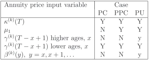
Evaluation of equation (5) requires knowledge of: β(k)(x), β(k)(x+ 1), . . .; κ(k)(T);
µ1; and the single cohort effect, γ(k)(T −x+ 1). The questions, therefore, arise as
to how and when we estimate these various inputs. We consider three cases: full parameter certainty; partial parameter certainty; full parameter uncertainty.
In all three cases, we will calibrate the model using the single-population version of the APC model given in equation (3) above. This model is fitted separately to each of the EW and CMI datasets, without making any assumptions about the time series properties of the age, period or cohort effects (that is, as in Cairns et al., 2009).
In the full parameters-certain (PC) case, we proceed in the following steps:
• PC1: Fit the one-population model to each of the EW and CMI datasets running from 1981 to 2005: this is referred to as the initial calibration and is required for PC4.
• PC2: Fit a random walk model to the fitted period effect (EW) for 1981 to 2005. This gives us the estimated random-walk drift,µI
1.
22A more sophisticated approach would allow for the initial drift ofκ(2)(t) to differ fromµ1, but then revert toµ1in the long run. Thus, in the expression for ˆmk(T+s, x), we might replaceµ2s byµ1s+ (µ2−µ1)(1−φs)/(1−φ) where φ >0 is the AR(1) parameter in the spread between
• PC3: Simulations from 2005 to 2015 are carried out using the PC version of the two-population model (see Cairns et al., 2011b, for details).
• PC4: For each stochastic scenario taking us from 2005 to 2015: refit the one-population model to each population, subject to the constraint that age, period and cohort effects already estimated in the initial calibration remain unchanged. This means that we estimate only the 10 most recent period and cohort effects.
• PC5: For each scenario, annuity valuation atT = 10 requires projection of the period effects only, and so we useκ(k)(T) resulting from the time-T calibration,
and the random-walk drift, µI
1, that was already estimated at time 0.
In the partial-parameters-certain (PPC) case, we proceed as follows:
• PPC1 to PPC4: Same as PC1 to PC4.
• PPC4A: Recalibrate the random-walk parameter values for the single-population period effect, κ(k)(t), using the W most recent values: in particular, we
re-calibrate the drift parameter,
µ1 =
¡
κ(1)(T)−κ(1)(T −W)¢
/W.
This is in contrast with the PC case, where µ1 is left equal to its initial
cali-bration, µI
1.
• PPC5: For each scenario, annuity valuation at T = 10 requires projection of the period effects only, and so we use κ(k)(T) resulting from the time-T
calibration, and the recalibrated random-walk drift,µ1.
In the full parameters-uncertain (PU) case, we proceed as follows:
• PU1/2: Not required.
• PU3: Simulations from 2005 to 2015 are carried out using the the PU version of the two-population model (see Cairns et al., 2011b, for details).
• PU4: For each stochastic scenario taking us from 2005 to 2015, use the historical-plus-simulated deaths and exposures to carry out a full recalibra-tion (in contrast with partial recalibrarecalibra-tion in PC4 and PPC4) of the single-population APC models to the EW and CMI single-populations using actual deaths and exposures over a window of W + 1 years (i.e., calendar years T −W to
T).
• PU4A: Recalibrate the random-walk parameter values for the single-population period effect, κ(k)(t), using the W most recent values: in particular, we
re-calibrate the drift parameter,
µ1 =
¡
κ(1)(T)−κ(1)(T −W)¢
Annuity price input variable Case PC PPC PU
κ(k)(T) Y Y Y
µ1 N Y Y
γ(k)(T −x+ 1) higher ages, x N N y
γ(k)(T −x+ 1) lower ages, x Y Y Y
[image:20.595.165.426.96.202.2]β(k)(y), y=x, x+ 1, . . . N N y
Table 4: Input factors as a source of risk in the calculation of the annuity price,
ak(T, x). N: no, the variable is fixed at time t = 0 (end 2005). Y: yes, variable is
not known until time T, and is a significant source of risk. y: the variable can be estimated at t = 0, but is also subject to estimation uncertainty, and is subject to modest amounts of re-calibration risk atT.
• PU5: For each scenario, annuity valuation atT = 10 requires projection of the period effects only, and so we useκ(k)(T) resulting from the time-T calibration,
and the recalibrated random-walk drift,µ1.
5.4
The recalibration window,
W
+ 1
In the PPC and PU cases, µ1 uses a recalibration window of W years up to timeT
to estimateµ1. In this paper, we will assume in most of our numerical experiments
that W + 1 = 20 years. However, we will later discuss the sensitivity of the results to the choice of W.
5.5
Sources of uncertainty in
a
k(
T, x
)
At the beginning of this section, we identified the various inputs required for the calculation of ak(T, x). We now consider which of these inputs causes uncertainty
inak(T, x) (see, also, Table 4):
• κ(k)(T) constitutes the principal source of randomness in a
k(T, x). It is the
only source of uncertainty in the full PC case for all but the lowest ages at time T (i.e., ages at time T with cohort effects that had not been estimated at time 0).
• In some cases, the value ofγ(k)(T+ 1−x) used in the calculation ofa
k(T, x) is
uncertain. Specifically, this is the case for younger ages, x, starting with the cohort aged x0 +T at the end of year T (where x0 = 50 is the youngest age
in our data) down to the cohort agedx0 at the end of year T. None of these
cohorts was included in the dataset available at time 0 (i.e. 2005), and so the relevant value of γ(k)(T + 1−x) is uncertain and not measurable until some
• In the full PC case, there are no further sources of uncertainty. At time T, only the T most recent period and cohort effects are estimated; parameters already estimated at time 0 are left as they are; and the value of µ1 is left
unchanged from its initial calibration at time 0.
• In the PPC case, the estimated age, period and cohort effects are treated as known and not subject to parameter estimation uncertainty. In contrast with the full PC case, however, the random walk drift, µ1, is recalibrated at time
T, based on estimates of the period effectκ(1)(t) up to time T, and this means
that µ1 in the calculation of the ak(T, x) is uncertain.
• In the PU case, individual sample paths take account of parameter uncertainty in the 2005 calibration and the model is fully recalibrated at time T. Thus, besides the process risk inherent in the period up to timeT and cohort effects for younger ages, full recalibration at T plus PU at t = 0 means that the
β(k)(x) and γ(k)(c) inputs to a
k(T, x) are also uncertain.
6
Decomposing hedge effectiveness in customised
and index longevity hedges
Basis risk and, therefore, hedge effectiveness are influenced by the risk factors out-lined in section 1.1 above. We will now examine what we believe to be the most important risk factors that impact on the hedge effectiveness of longevity hedges, namely population basis risk, cohort effect uncertainty, recalibration risk, recalibra-tion window, parameter uncertainty, and Poisson risk. We do this using the example of a pension plan that is considering employing either a customised or index value hedge as part of an asset-liability management exercise.
6.1
Correlation results for individual risk factors
We now take a detailed look at how the correlation between the liability and the hedging instrument values changes in response to the inclusion or exclusion of the various factors listed in the previous section. To recap: our liability value isL(T) =
a2(T, x), where T = 10 (2015) and x = 65, and our hedging instrument value is
H(T) =ak(T, y)−ˆaf xdk (T, y) where, again, T = 10, but y can range from 50 to 89,
and the reference population might be either k = 1 (index-based hedge) or k = 2 (customised hedge).
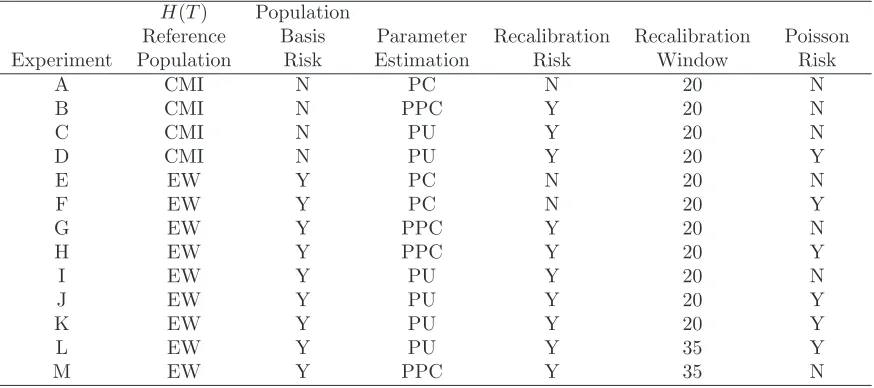
reference age, y. In all, Figures 1 to 7 cover 13 experiments (A to M) that are outlined in Table 5.23 We are primarily interested in the effectiveness of index
hedges, although, in most cases, we also plot the equivalent correlation curve for a customised hedge allowing us to compare the impact of the various risk factors on each type of hedge.
H(T) Population
Reference Basis Parameter Recalibration Recalibration Poisson Experiment Population Risk Estimation Risk Window Risk
A CMI N PC N 20 N
B CMI N PPC Y 20 N
C CMI N PU Y 20 N
D CMI N PU Y 20 Y
E EW Y PC N 20 N
F EW Y PC N 20 Y
G EW Y PPC Y 20 N
H EW Y PPC Y 20 Y
I EW Y PU Y 20 N
J EW Y PU Y 20 Y
K EW Y PU Y 20 Y
L EW Y PU Y 35 Y
[image:22.595.83.520.192.386.2]M EW Y PPC Y 35 N
Table 5: Key risk factors influencing the correlation between liability and hedge values for experiments A to M. The cohort effect, as a source of risk at younger ages, is present in all experiments. All experiments involve life annuities apart from experiment K which uses a temporary annuity that ceases at age 90.
To help with the interpretation of the results, it is useful to consider a linear approx-imation of the annuity price. First, note that ak(T, x) =f(β(k)[x], κ(k)(T), γ(k)(T −
x+ 1), µ1), where β(k)[x] is the column vector of age effects from age x upwards,
(β(k)(x), . . . , β(k)(ω))′
,ω is the maximum age, andf(·) is the annuity function gov-erned by the deterministic projection of the period effects. The linearisation is then simply:
ak(T, y) ≈ f( ˆβ(k)[x],κˆ(k)(T),ˆγ(k)(T −x+ 1),µˆ1)
+b′
1(y)
³
β(k)[x]−βˆ(k)[x]´+b 2(y)
³
κ(k)(T)−κˆ(k)(T)´
+b3(y)
³
γ(k)(T −x+ 1)−γˆ(k)(T −x+ 1)´+b4(y)
³
µ1−µˆ1
´
. (6)
This linearisation turns out to be a very accurate approximation to f(·), even with full PU and uncertainty in all of the β(k)[x], κ(k)(T), γ(k)(T −x+ 1), and µ
1.
Turning now to the experiments listed in Table 5:
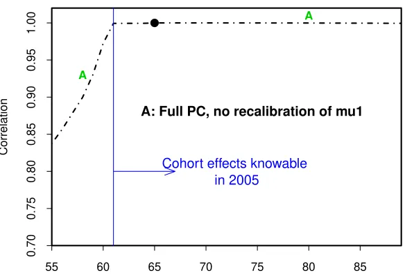
• Benchmark customised hedge: To provide a reference point, we start with a benchmark customised hedge (Figure 1). We take the simplest case, namely
full parameter certainty (PC) without Poisson risk. The correlation curve (A) has two distinct parts to it. At ages 61 and above, the correlation is both very flat and very close to 1. In the PC case,L(T) andH(T) have κ(2)(T) as their
single source of randomness, so the correlations are almost 1 (‘almost’ because there are still some slight non-linearities).24
• Cohort effect uncertainty:25 Also in Figure 1, we note that the correla-tions drop away below age 61. This is because a2(T, y) also depends on the
cohort effectγ(2)(c) for year of birth, c=T −y+ 1. If the hedging instrument
reference age,y, is less than 61, then the relevant value of γ(2)(c) is not known
until after 2005 and therefore provides an additional source of randomness in
H(T). As we move from age 61 to younger ages (i.e., later years of birth), uncertainty in γ(2)(c) grows and, therefore, makes an increasing contribution
to the overall risk in H(T). Since this additional risk is not correlated with
κ(2)(T), the correlation between H(T) and L(T) falls in line with the
propor-tional contribution ofγ(2)(c) to the uncertainty in H(T).
• Population basis risk: In Figure 2, we introduce population basis risk by switching to the use of hedging instruments linked to the EW males population. We see that the broad impact of this switch is to pull down the correlation curve at all ages. Experiment E (dot-dashed line) gives correlations in the full PC case. As with curve A, curve E is fairly flat above age 61, reflecting the near-linear dependence of L(T) andH(T) on their single sources of risk,
κ(2)(T) and κ(1)(T), respectively. This dependence is confirmed by the fact
that Cor(L(T), H(T))≈Cor(κ(1)(T), κ(2)(T)) above age 61.
• Recalibration risk: Figure 3 shows the impact of model recalibration risk in the PPC case for both the customised (A to B) and index (E to G) hedges. First, consider customised hedges. This introduces a fresh source of risk, µ1,
into the calculation of annuity values. In experiment B (solid curve), above age 61, there are two distinct sources of risk (κ(2)(T) andµ
1, which, as previously
discussed, is a linear function ofκ(1)(T)). Over the 61+ age range, correlations
are still high, but, asyincreases above age 65, correlations drift down gradually (curve B). For y close to age 65, L(T) and H(T) are exposed to the κ(2)(T)
and µ1 risks in approximately the same proportions (i.e., the ratio of b2(y) to
b4(y) in equation (6)). However, as the reference age, y, increases, the relative
impact of κ(2)(T) and µ
1 on a2(T, y) changes (i.e. b2(y) to b4(y)), causing
correlations to drop a little (solid line (B), right-hand end).
Below age 61, in experiment B, there are three sources of risk: κ(2)(T),µ 1 and
γ(2)(T −y+ 1). The curve drops away as we reduce y for similar reasons as
24In this experiment, onlyκ(2)(T) is uncertain in the linearised equation (6), so the correlations betweena2(T, x) anda2(T, y) in the linearised version forx6=y must be exactly equal to 1.
in experiment A. However, it is obvious that correlations for these lower ages are much higher in experiment B compared with A. In experiment B, L(T) and H(T) have, in absolute terms, significantly more risk than A, through additional uncertainty in µ1. However, in relative terms, L(T) and H(T)
have a much stronger dependence on common sources of risk (κ(2)(T) and
µ1) in experiment B than in experiment A and this results in a much higher
correlation.
Now consider the impact of recalibration risk on an index hedge. As a source of risk, µ1 is common to both L(T) and H(T) over all reference ages. The
inclusion of recalibration risk significantly increases the uncertainty in L(T) andH(T), but this is a perfectly correlated additional risk.26 Thus, the impact
of including PPC model recalibration risk is to increase the correlations and so raise curve E (dot-dashed line) significantly to curve G (solid line).
Finally, in Figure 3, we compare experiments E (PC) and G (PPC) below age 61. In the PPC case (G), at lower ages, the additional risk in the cohort effect (Figure 8) is just as large in absolute terms as the full PC case (E), but, in relative terms, it contributes much less, because of the inclusion of the additional risk linked to µ1 that is common to both L(T) and H(T). As a
result, the decline in correlations below age 61 is less in the PPC case (G).
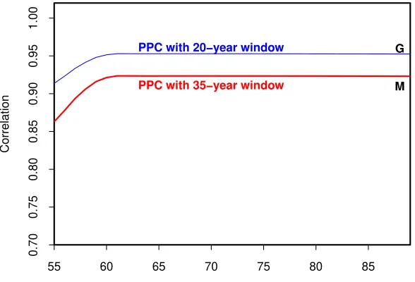
• Recalibration window: In Figure 4, we focus on the sensitivity of results to the choice of recalibration window. In experiment G, we use a 20-year window and, in experiment M, we use a 35-year window. Recall that µ1 =
(κ(1)(T)−κ(1)(T −W))/W, so W + 1 = 35 rather than W + 1 = 20 reduces
uncertainty inµ1. Comparing experiments G and M, bothL(T) andH(T) are
less risky under M, becauseµ1 is less risky. However, the correlation between
L(T) and H(T) is also now lower because of their greater dependence, in relative terms, on the imperfectly correlated κ(2)(T) and κ(1)(T).
• Parameter uncertainty: Figure 5 adds in the impact of parameter uncer-tainty (PU) (experiments C and I, dashed lines). Introducing PU creates additional uncertainty in the process parameters (e.g., µ1) and also in the
latent state variables (the age, period and cohort effects). This additional un-certainty can be thought of as noise on top of the main signal and the noise added to the different components ofL(T) and H(T) will be largely uncorre-lated.27 This creates additional risk that is mostly non-hedgeable (with the
exception of age 65, where L(T) and H(T) refer to the same cohort) and so leads to lower correlations and lower hedge effectiveness.
26Referring to equation (6),L(T) is approximately a linear combination ofκ(2)(T) andµ1, while
H(T) is a linear combination ofκ(1)(T) and µ1. In the PPC case, µ
1 is a risk that is common to bothL(T) andH(T) and so raises the correlation between the two relative to the PC case, where
µ1is fixed.
27For example, the noise added to κ(1)(T) and κ(2)(T) will have a low correlation, and, for
Figure 5 also shows the impact of moving from the PPC (curve G) to the PU case (curve I, dashed line) on the effectiveness of an index hedge. The impact is relatively small, with a magnitude that is similar at most ages to the customised hedge (experiments B and C). However, in contrast with the shift from B to C, we find here that there is no advantage to using a hedging instrument that is linked to exactly the same birth cohort as the liability being hedged: this reflects a lack of correlation in the PU setting between our estimates of the cohort effects in the two populations, γ(2)(T − x+ 1) and
γ(1)(T −x+ 1) for x= 65.
• Poisson risk: In Figure 6, we look at the impact of adding in Poisson risk (experiments D and J, dotted lines). In general, this should add to the uncer-tainty in bothL(T) andH(T).28 The impact on correlation of Poisson risk (C
to D) is broadly similar in magnitude to the impact of PU (B to C). However, the impact does seem to vary with age. The reasons for these variations are not clear, suggesting that the impact of Poisson risk on the various inputs to
a2(T, y) is complex. In contrast (experiments I and J), if we use an
index-based hedge, then the gap between the Poisson and no-Poisson correlation plots seems to be reasonably uniform across all ages.
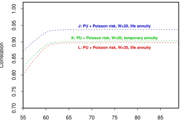
• Term of the annuity: In Figure 7, we make two further comparisons. As our baseline, we conduct experiment J which includes all risk factors. We investigate how sensitive the correlations are to the term of the annuity that underpins our calculations. Experiment J involves the use of a life annuity. In contrast, in experiment K, both L(T) and H(T) involve temporary annuities that cease at age 90. We can see that this lowers the correlations relative to curve I. This is explained by the fact that the recalibrated µ1 has relatively
little influence over short-dated cashflows and much greater influence over long-dated cashflows. By shifting to temporary annuities, we have therefore reduced the influence of µ1 on L(T) and H(T), with a resulting lowering in
the correlations.
A similar shift would occur if we switched from a life annuity starting at age 65 to, say, a life annuity starting at age 75, since, on average, the annuity will be payable for less time.
• Recalibration window revisited: In Figure 7, which shows the results of experiment L, we repeat the shift from a recalibration window of 20 to one of 35 years, this time in a full PU setting with Poisson risk (compare with Figure 4.) The difference between J and L can be seen to be similar to (but slightly larger than) the shift from G to M. Thus, the impact of a change in the recalibration window can be seen to be not especially sensitive to the inclusion or otherwise of the less important risk factors (full PU and Poisson risk).
55 60 65 70 75 80 85
0.70
0.75
0.80
0.85
0.90
0.95
1.00
Cohort effects knowable in 2005
A
A
A: Full PC, no recalibration of mu1
Hedging Instrument Reference Age, y
[image:26.595.148.440.112.314.2]Correlation
Figure 1: Correlation between the liability, L(T), and hedging instrument, H(T), values as a function of the hedging instrument reference age. Experiment A (Table 5) assumes a customised hedge (CMI reference population), full parameter certainty (PC) and no Poisson risk. Knowable cohort effects are discussed in Appendix C. The black dot identifies the liability reference age of 65.
55 60 65 70 75 80 85
0.70
0.75
0.80
0.85
0.90
0.95
1.00
+ Population basis risk E
A
A
Hedging Instrument Reference Age, y
Correlation
[image:26.595.149.442.454.653.2]55 60 65 70 75 80 85
0.70
0.75
0.80
0.85
0.90
0.95
1.00
E
A
A B
B
G
Hedging Instrument Reference Age, y
[image:27.595.148.444.114.313.2]Correlation
Figure 3: Correlation between the liability, L(T), and hedging instrument, H(T), values as a function of the hedging instrument reference age. Experiments A, B, E, G (Table 5). A, B: customised hedges. E, G: index hedges. A, E: full PC. B, G: PPC with recalibration risk, 20-year recalibration window. All: without Poisson risk.
55 60 65 70 75 80 85
0.70
0.75
0.80
0.85
0.90
0.95
1.00
M G
PPC with 20−year window
PPC with 35−year window
Hedging Instrument Reference Age, y
Correlation
[image:27.595.147.441.451.651.2]55 60 65 70 75 80 85
0.70
0.75
0.80
0.85
0.90
0.95
1.00 B C B
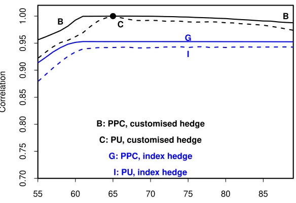
G
I
B: PPC, customised hedge
C: PU, customised hedge
G: PPC, index hedge
I: PU, index hedge
Hedging Instrument Reference Age, y
[image:28.595.148.440.116.317.2]Correlation
Figure 5: Correlation between the liability, L(T), and hedging instrument, H(T), values as a function of the hedging instrument reference age. Experiments B, C, G, I (Table 5). All: without Poisson risk; 20-year recalibration window. B, C: customised hedges. G, I: index hedges. B, G: PPC. C, I: full PU.
55 60 65 70 75 80 85
0.70
0.75
0.80
0.85
0.90
0.95
1.00 C
D C
D
I
J
C: PU, customised hedge
D: PU, customised hedge + Poisson risk
I: PU, index hedge
J: PU, index hedge + Poisson risk
Hedging Instrument Reference Age, y
Correlation
[image:28.595.146.440.442.641.2]55 60 65 70 75 80 85
0.70
0.75
0.80
0.85
0.90
0.95
1.00
J: PU + Poisson risk, W=20, life annuity
K: PU + Poisson risk, W=20, temporary annuity
L: PU + Poisson risk, W=35, life annuity
Hedging Instrument Reference Age, y
[image:29.595.148.441.272.471.2]Correlation
6.2
Analysis
Our discussion above of the individual plots focused on the incremental impact of the different risk factors. Here we look at the bigger picture and assess the overall impact and significance of each, beginning with the most important.
• Population basis riskis clearly a very significant factor. However, its negative impact on correlation and hedge effectiveness is not, perhaps, as large as might seem at first glance.
• Recalibration riskis also a factor of potential significance, although its precise impact depends on the type of hedge. For index hedges, it results in substan-tially increased correlations and hence hedge effectiveness;29 for customised
hedges, it has a very modest, negative impact.
Further, as demonstrated in Figure 7, the impact of recalibration risk will be more substantial30 if both the liability and hedging instrument values (in an
index hedge) depend more heavily on more distant longevity-linked cashflows. In relative terms, these cashflows are much more sensitive to changes in the random-walk drift µ1.
• The impact of recalibration risk on correlations was found to be quite sensitive to the length of the calibration window (e.g. 20 years or 35 years): a longer calibration window lowers correlation and hedge effectiveness.
• Cohort effect uncertaintycan cause correlations to be pulled down if the liabil-ity and hedging instrument refer to different cohorts either by year of birth or by reference population. The impact is modest if both of the relevant cohort effects had been estimated at time 0 (2005), and is a result of uncertainty in the estimates of those state variables. The impact is much more significant if one or other of the relevant cohort effects could not be estimated in 2005, thereby introducing additional uncertainty in the calculation of the annuity price atT.
• Where we have already taken account of recalibration risk, the inclusion of other forms of parameter uncertainty (PU) and Poisson risk only have a mod-est impact on correlation and hedge effectiveness. However, if the underlying populations were much smaller than those considered here, then PU and Pois-son risk are likely to have a bigger impact.
29Where allowance for recalibration risk does increase correlations and hedge effectiveness, this helps to explain why the negative impact of population basis risk is smaller than anticipated.
7
Conclusions
This paper builds on the framework proposed by Coughlan et al. (2011) by analysing hedge effectiveness (with correlation as a proxy) using stochastic simulation (instead of historical bootstrapping). It is the first study to bring together, in a single stochas-tic modelling framework, the key risk factors influencing the effectiveness of longevity hedges, namely population basis risk, cohort effect uncertainty, recalibration risk, recalibration window, parameter uncertainty and Poisson risk.
To investigate longevity hedge effectiveness, we used a case study of a pension plan that wishes to hedge the value of its liability in 10 years’ time to a male member who is currently aged 55. The liability is therefore equivalent to a deferred annuity. The plan had the choice of using either a customised hedge or an index hedge. We assumed, for the sake of illustration, that the mortality experience of the pension plan and the customised hedge was the same as the Continuous Mortality Investi-gation’s male assured lives, while the mortality experience of the index hedge was the same as that for the England & Wales male population. For such hedges, we showed that correlation is a good measure of hedge effectiveness.
We found that population basis risk and uncertain future cohort effects are signif-icant determinants of hedge effectiveness. However, we also showed that this was just the starting point. We discovered that correlation and hedge effectiveness are also affected to a significant extent by the inclusion of recalibration risk and the assumed length of the recalibration window. Beyond that, further sources of pa-rameter uncertainty and Poisson risk have a more modest, although still noticeable, impact. However, we argue that the latter two sources of risk would have a greater impact if one or both of the populations were much smaller than those considered here.
The strong conclusion is that an analysis that ignores parameter uncertainty (includ-ing recalibration risk) might significantly underestimate the level of longevity risk, but, more importantly, might also underestimate the degree of hedge effectiveness of an index-based longevity hedge. So an unsophisticated and incomplete analysis of the problem might either lead to a decision not to hedge (because the level of risk is deemed not to be sufficiently high) or lead to a customised hedge being chosen in place of a cheaper index hedge (because the effectiveness of the latter has been underestimated).
Our case study shows that longevity basis risk can be substantially hedged using index hedges as an alternative to customised longevity hedges. As a consequence, therefore, index longevity hedges – in conjunction with the other components of an ALM strategy – can provide an effective as well as a low cost alternative to a full buy-out of pension liabilities or even a strategy that involves the use of customised longevity hedges.
to investigate such factors as the type of hedging instrument (namely, alternatives to a deferred longevity swap), the optimality and robustness of the hedge ratio, value versus cashflow hedges, static versus dynamic hedges, and the use of multiple hedging instruments, etc. Also omitted is an analysis of the impact of model risk: a substantial topic in its own right. Finally, we have not analysed the sensitivity of longevity hedge ratios to changes in the underlying assumptions. We leave these issues for future work.
References
Blake, D., and Burrows, W. (2001) Survivor bonds: Helping to hedge mortality risk.
Journal of Risk and Insurance, 68: 339-348.
Blake, D., Boardman, T., and Cairns, A.J.G. (2010) Sharing longevity risk: Why governments should issue longevity bonds. Pensions Institute Discussion Paper PI1002 (accessed on 14/4/2011 at
http://www.pensions-institute.org/workingpapers/wp1002.pdf).
Blake, D., Cairns, A.J.G., and Dowd, K. (2006) Living with mortality: Longevity bonds and other mortality-linked securities. British Actuarial Journal, 12: 153-197.
Brouhns, N., Denuit, M., and Vermunt J.K. (2002) A Poisson log-bilinear regression approach to the construction of projected life tables. Insurance: Mathematics and Economics, 31: 373-393.
Cairns, A.J.G., Blake, D., and Dowd, K. (2006) A two-factor model for stochastic mortality with parameter uncertainty: Theory and calibration. Journal of Risk and Insurance, 73: 687-718.
Cairns, A.J.G., Blake, D., and Dowd, K. (2008) Modelling and management of mortality risk: A review. Scandinavian Actuarial Journal, 2008(2-3): 79-113.
Cairns, A.J.G., Blake, D., Dowd, K., Coughlan, G.D., Epstein, D., Ong, A., and Balevich, I. (2009) A quantitative comparison of stochastic mortality models using data from England & Wales and the United States. North American Actuarial Journal, 13: 1-35.
Cairns, A.J.G., Blake, D., Dowd, K., Coughlan, G.D., Epstein, D., and Khalaf-Allah, M. (2011a) Mortality density forecasts: an analysis of six stochastic mortality models. Insurance: Mathematics and Economics, 48: 355-367.
Cairns, A.J.G., Blake, D., Dowd, K., Coughlan, G.D., and Khalaf-Allah, M. (2011b) Bayesian stochastic mortality modelling for two populations, To appear in ASTIN Bulletin.