Gulag, WWII and the Long run Patterns of Soviet City Growth

Munich Personal RePEc Archive

Gulag, WWII and the Long-run Patterns

of Soviet City Growth

Mikhailova, Tatiana

New Economic School, Center for Market Studies and Spatial

Economics, Higher School of Economics

9 September 2012

Online at

https://mpra.ub.uni-muenchen.de/41758/

Gulag, WWII and the Long-run Patterns of Soviet City

Growth

Tatiana Mikhailova

September 9, 2012

Abstract

This paper analyzes the geographical patterns of city growth in the Soviet Union and the Russian Federation in relation to the Stalinist policies of the 1930s to 1950s, and WWII. Using a unique data set on the locations of Gulag camps, and on the evacuation of industrial enterprises during WWII, I estimate the effect of these factors on city growth throughout the Soviet and post-Soviet period. The cities where Gulag camps were located grew significantly faster than similar cities without camps. WWII events (location of the frontlines, evacuation) also affected local population growth, but their impact diminished with time and disappeared completely after 25 years. In contrast, the effect of Gulag camps has been permanent.

First version: October 2011 Preliminary and incomplete

JEL classification: R11, R12, P25 Keywords: Cities, USSR, Gulag, WWII

Address: Nakhimovsky pr., 47, Suite 1721, Moscow, Russia 117418. E-mail: [email protected]

∗_{New Economic School and the Center for Theory of Markets and Spatial Economics, Higher School of}

1

Introduction

Over the twentieth century the territorial distribution of economic activity and productive resources in the Soviet Union and Russia has changed dramatically. Both historical events and Soviet policies – notably the devastation of western parts of the USSR and the evacuation of people and enterprises during WWII, re-evacuation and reconstruction after the war, Stalin’s industrialization and the build up of the industrial capacity east of the Urals, and Gulag, kulak and ethnic deportations – were driving these spatial shifts.

Still, largely because of the lack of of detailed data, we do not know much about how these historical events and policies changed the economic geography of the USSR and Russia. Were their effects short-lived, or did they persist over a long time? Could they still be economically relevant today? More generally, should we expect a return to a “normal” path of development after any exogenous shock, such as a war or “forced” policy, or can some of the shocks or policies be so drastic that they permanently affect the spatial development path?

In this paper, I analyze the patterns of city growth in the Soviet Union and the Russian Federation by constructing a unique dataset on the location of Gulag camps and the evacua-tion of industrial enterprises during WWII, and then matching those camps and enterprises to the nearest urban settlements. I therefore estimate the effect of WWII, evacuation, and Gulag camps on population growth in Soviet cities over a long time horizon. To my knowl-edge, this is the first paper that looks at both Gulag and wartime events in the context of regional population growth in the USSR using city-level data.

Working with city-level data allows me to investigate the spatial patterns of development on a much finer scale and over a much longer time horizon. While sub-regional and regional administrative boundaries have changed a lot during the Soviet history, cities are clearly defined administrative units. With a panel of city-level data for a long historical period, I can investigate the heterogeneity in population growth both between and within regions.

population growth in Soviet cities. WWII events (fighting on the front, evacuation) also affect local population growth, but their effects are relatively short-lived, diminishing with time and disappearing after about 25 years. In contrast, the Gulag camps have a permanent effect on city size. The cities where camps were located grew significantly faster and continued to grow faster long after the Gulag system itself was abolished.

This paper adds to two strands of the literature, the first of which is the literature on population geography and industrial location in the USSR and the Russian Federation. A number of existing papers analyze regional investment patterns and population growth over the different periods of Soviet history: Hooson (1968) describes patterns of city growth prior to and after the October revolution; Harrison (1988) and (1990) discuss the reallocation of the Soviet industry to the eastern regions of the USSR prior and during the WWII; the ideological principles of Soviet location policy and their actual realization were considered in Dienes (1972), Dyker (1983), Huzinec (1977), and Rodgers (1974), among others; Andrienko & Guriev (2004) and Kumo (2006) studied interregional migration flows in Russia after transition.

The existing literature on Soviet economic geography relies mainly on region-level data analysis, except for the analysis of Soviet population dynamics by Gang & Stuart (1999) and Iyer (2003). Gang & Stuart (1999) study the growth of cities in terms of migration restrictions in the USSR during the period from the 1930s to the 1980s. They find little or no effect of these restrictions on population growth. I confirm their results for the wider sample of cities, with more recent data, and a different methodology. Iyer (2003) looks at the rank-size distribution of Russian cities and finds an increasing concentration of urban population after the transition to a market economy.

in one location, it is difficult to change the spatial allocation of productive resources, even if an alternative location is equally (or even more) suitable for concentrated economic activity. Only large shocks to the spatial structure of the economy have the potential to trigger a switch between equilibria. By looking at the wartime and post-war data, researchers can observe how population and industrial geography change after a significant exogenous shock, and determine whether wartime destruction can indeed trigger the switch between spatial equilibria.

Davis & Weinstein (2002) and (2008) investigate the long-term dynamics of popula-tion and industry locapopula-tion after the shock of WWII destrucpopula-tion in Japan using city-level data. Brakman, Garretsen & Schramm (2004) and Bosker, Brakman, Garretsen & Schramm (2007) look at German cities after WWII. Miguel & Roland (2011) look at the regions of Vietnam and their recovery after U.S. bombing. In this literature, one common finding is that wartime destruction has little or no effect on regional patterns of population growth, industrial geography, or regional development in the long run. Regional population levels tend to recover within 15-25 years after a shock. While this is true for Japan and Vietnam, West Germany exhibits only partial reversion toward the pre-war levels. The robustness of this result may suggest that the multiplicity of equilibria is either a purely theoretical notion that does not normally occur in reality, or that even drastic wartime shocks are not large enough to motivate a switch between equilibria.1

So far, the division of Germany after WWII is the only historical event researchers have studied in which an exogenous shock resulted in permanent changes to the spatial economy landscape. Redding, Sturm & Wolf (2011) find evidence of a multiplicity of equilibria in the location of Germany’s air travel industry. The switch of equilibrium was triggered by the post-WWII division of Germany, but its reversal was not triggered by the reunification of Germany in 1990. Redding & Sturm (2008) find persistent long-term negative effects of Germany division for the West German cities near the newly established border with Eastern

1

Germany. It is not wartime destruction that affected the relative sizes of German cities in the long run, but rather the changes in their market access (market potential).

The Soviet Union presents a unique case for studying the effects of war on the spatial economy and radical regional policy. On one hand, like many other countries the USSR suffered direct effects of WWII: destruction of its capital and infrastructure and loss of lives. On the other hand, during the 1930s to 1950s while capital and infrastructure in the USSR were destroyed in the western regions they were being built up in the other parts of the country, mainly in the east. Relocating people and capital across the country, Stalin used policy to create industrial centers from scratch in places where they would hardly have emerged as the result of free migration of small economic agents (people, firms) in a market economy. Similar to the division of Germany, this served as a shock to market potential, but it was a different type of shock: agglomeration externalities were not exogenously destroyed (as in case of cities on the border between West and East Germany), but rather were created. My findings on the effects of the war confirm the earlier literature: the impact of wartime destruction, however devastating it might have been, was temporary. On average, Soviet cities affected by the war eventually recovered. In contrast the Gulag, like the division of Germany, presents an example of permanent change in the spatial economy landscape. Redding et al. (2011) point out that even if multiple equilibria in industrial location are possible, in order to switch equilibria the shock to industrial location has to be not only strong but also perceived by economic agents as permanent. Soviet location policy (as proxied by Gulag) is a perfect example of such a significant change which was thought to be permanent at the time.

2

The History of Gulag, Wartime Evacuation, and the

Spatial Evolution of the Soviet Economy

Gulag

Gulag (a collection of penitentiary institutions) has its roots in the Russian Civil war period of 1917-1922. The first concentration camps, where prisoners’ labor was used for “community service,” were established as early as 1919. In the beginning, the primary purpose of these camps was punishment, not economic activity. That doctrine changed as the 1930s began. Ivanova (2006) cites a joint memo from the People’s Commissariats of Justice and the Interior and the Joint State Political Directorate (OGPU) to the Council of People’s Commissars of the RSFSR dated April 1929 proposing “1. To use prisoners serving a term of 3 years or more in colonization of our northern frontier territories and in developing the natural

resources there.”2

Thus Gulag became a tool of regional development in the early 1930s. At the same time, the number of camps and the total prisoner population began to grow rapidly, from 179 thousand prisoners in 1930 to almost 1.9 million in 1938.3

Gulag population continued to grow steadily until Stalin’s death, with the peak number of prisoners, 2.5 million, in 1952. From 1935 to 1952, the Gulag system was responsible for 6-10% of all construction in the USSR.4

Figure 1 illustrates the geographical location of the Gulag camps. Although originally in remote locations, camps eventually were organized in practically all areas of the country. In fact, a Gulag map looks much like the map of population density.

The largest camps were established at the sites of major infrastructure projects that required a lot of labor. Not all of these camps were in the remote areas; of the ten biggest camps, six were west of the Ural mountains and three were in or near major cities. Table 1 gives some examples of the location and major activities of the largest camps.

2

Author’s translation, source: Ivanova (2006), page 161.

3

Data compiled from NKVD documents, cited in many sources, including Applebaum (2003).

4

Source: Smirnov (1998), map online at www.memo.ru.

Figure 1: Gulag camps in the USSR.

Max capacity,

thousand Capacity Years of

Camp name Location people rank operation Primary activity Svobodnyi, Amur oblast

Baikal- 110 km north-east of Construction of

Baikal--Amur ITL∗ _{Blagoveshensk 201 1 1932-1938 Amur railroad}

Severo- 330 km north

-Vostochnyi ITL of Magadan 190 2 1932-1949 Gold mining

Dmitrov, 50 km north Construction of

Moscow-Dmitrovsky ITL of Moscow 189 3 1932-1938 Volga canal

Dalne- Railroad construction,

-Vostochny ITL Khabarovsk 112 5 1929-1939 coal mining, gold mining

Belomoro- Medvezh’egorsk, 120 km Construction of

-Baltiisky ITL north of Petrozavodsk 108 6 1931-1941 ”Belomorkanal” Construction of

Rybinsk, 83 km north- hydroel. power plant and

Volzhskii ITL -west of Yaroslavl 88 8 1935-1942 canal infrastructure Bezymyanskii

ITL Samara 81 9 1941-1946 Industrial construction

Mariinsk, 130 km north- Logging,

Sibirskii ITL -east of Kemerovo 78 11 1929-1960 road construction

*”ITL” is a transliteration of a Russian acronim forispravetelno-trudovoi lager’ (correctional labor camp).

A stereotype of a Gulag camp is a remote location with a hostile climate and no infras-tructure, but looking at the newly systematized data on camp locations paints a different picture.5

A vast majority of the camps operated in or near cities or towns. Figure 2 shows the distribution of camps in terms of distance to the nearest population center with the status of city: 83% of all camps were located no more than 35 kilometers from a settlement with city status now, and 66% of all camps were no more than 35 kilometers from a city of at least 10,000 inhabitants in 1939 (Figure 3). Thus, we can effectively conclude that Gulag was mainly an urban phenomenon.

Figure 2: Number of Gulag labor camps by the distance to the nearest population center.

Camps tended to be located near larger cities. If we compare the distributions of cities with and without Gulag camps nearby, we can see (in Figure 4) that the histogram of city sizes is heavier on the right tail for the group of cities with Gulag. Remote camps, and camps near small settlements, on average were larger by capacity (number of prisoners), but that correlation was not very strong (see Figure 5).

In general, as a tool of regional policy Gulag helped to shift productive resources from the

5

Figure 3: Number of Gulag labor camps by the distance to the nearest population center of 10 000 people or more in 1939.

Figure 4: Cities with Gulag camps nearby vs. all cities, 1939.

Figure 5: City size in 1939 and total max capacity of Gulag camps in 50 km radius.

its sheer amount of “cheap” prison labor allowed for the initiation of investment projects that hardly would have been possible had the Soviet government have to recruit voluntary labor there. Numerous documents underline the shortage-of-labor motivation in the creation and expansion of Gulag camps.6

Thus, geographically, the presence of a Gulag camp near a city or town points to a local deficit of voluntary labor in the 1930s to 1950s. This deficit, of course, was artificially created by Soviet planning itself and existed because of state-controlled wages. In fact, Gulag camp may be a good indicator that some investment project was undertaken nearby, and that the location was favored by the Soviet government for industrial development.

6

WWII evacuation

The Soviet government7

evacuated production lines and people (with priority given to skilled industrial workers and engineers) from the western territories in the first days after the German invasion. Thus, the first years of WWII resulted in a significant shift in regional industrial structure, from both the destruction and from this evacuation. A number of cities in the Soviet East received a significant positive shock to productive capacity, population, and human capital. Evacuation was also a major shock to regional population shares.

To my knowledge, the geography of wartime evacuation has never been studied in detail because the data were not available to the public. In public discourse, evacuation was long viewed as one factor that fueled the development of the eastern regions.But in reality there was no statistical evidence one way or the other that the cities that received evacuated enterprises indeed grew faster, simply because the detailed data did not exist in the public domain. In addition to the unavailability of the data, there is another challenge in accounting for the effect of evacuation: it has to be disentangled from the effects of the Soviet location policy in general. Evacuation, and the sudden change in the Soviet economic geography that it brought, were not spatially random.

Harrison (1990) emphasizes Stalin’s conviction that his pre-war policies contributed greatly to the USSR’s victory. Lieberman (1983) also notes that from the beginning of 1930s, one of the goals of Stalin’s industrialization clearly was to build up industrial ca-pacity deep in the Soviet territory, in the Urals and eastward, where it would be safe from invasion. These plans were only successful to a certain degree. The western parts of the USSR were the traditional industrial core of the Russian Empire. It would be difficult to shift the industrial base away from regions with a relative abundance of installed capital and skilled labor. As Harrison (1990) argues, despite the efforts of the Soviet government, the shift of industry eastward prior to the war was insufficient from the defense point of view.

7

Of course, the hurried evacuation in the first months of the war was a dire necessity, but it was also a forced implementation of an existing plan.

One indirect piece of evidence for the “preexisting plan” argument is that many of the evacuated plants either never moved back or continued to operate at both the new and old sites after the war. Of the 1374 enterprises for which I have information, only 453 have a record of being reestablished in some form at the old site after or during the war. Most commonly in the case of restored enterprises, instead of one enterprise two were operating after the war: one at the old and one at the new site.

Many of the cities to which enterprises were evacuated also hosted Gulag camps (the correlation between indicators of evacuation and Gulag on territories far from the frontlines is 41%; in the Urals, it is 46%). Naturally, if Gulag prisoners could easily be used to relieve the local deficit of labor, than the enterprises should be evacuated to where labor was easier to find in the war economy. This also suggests that the geographical allocation of the evacuated enterprises correlated strongly with the pre-war allocation of investment.

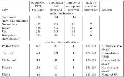
The summary statistics are: 1) enterprises were evacuated from 116 different cities to 190 different cities; 2) the main evacuation destinations were large cities – out of the top-20 destinations, 18 were oblast centers. However, many small settlements also received enterprises. Table 2 presents several examples of the destination cities and their population in the census years before and after the war. It was not uncommon for a city to increase its population by several hundred percent between these two censuses.

population population number of rank by 1939, 1959, enterprises the # of

City thousand thousand received enterprises location main destinations

Sverdlovsk 475 881 114 1

(now Ekaterinburg)

Novosibirsk 427 927 71 2

Kazan’ 418 647 66 3

Ufa 258 547 65 4

Kuibyshev 408 902 55 5

(now Samara)

smallest city-destinations

Pokhvistnevo 6.6 23 1 129-190 Kuibyshevskaia

oblast’

Tsivil’sk 5.1 5.9 1 129-190 Chuvashskaia

ASSR

Chebarkul’ 3.7 31 1 129-190 Cheliabinskaia

oblast’

Kataisk 2.8 12 1 129-190 Kurganskaia

oblast’

Ukhta 2.7 36 1 129-190 Komi ASSR

Table 2: Some examples of city-destinations in WWII evacuation.

3

Data

Population

The population data come from censuses in the Russian Empire (1897), the USSR (1926 -1989), and the Russian Federation (2002, 2010). For census years 1959 and 1939, the data come from Harris (1970); for all other years, from the original census publications. In all of the years, the sample includes all population centers with a city status and some of the larger rural settlements. 2002 and 2010 cross-sections include all urban population centers (cities and urban-type settlements) and rural settlements of 15000 or more.

Overall, the unbalanced panel has 9 time points (census years). The sample grows from 534 cities (uezdnye goroda) in 1897 to 2,002 cities and sizable rural settlements in 2010. Thirty-four small settlements with a city status are missing from the sample for 1926-1979 because they were omitted from the original publications.8

8

The administrative boundaries of a city in the USSR were not fixed. As cities grew, new land was added to the city territory, surrounding villages and small towns disappeared (in an administrative sense), being incorporated into larger population centers. Thus with the possible exception of the large agglomerations, the official city population data quite accurately reflect the size of an integrated urban economic area. For Moscow, St. Peters-burg, EkaterinPeters-burg, Novosibirsk, and Nizhnii Novgorod, I calculate the population of the agglomeration area, including all satellite cities and towns within a 30 km radius.

Gulag Camps

The main source of data for Gulag prisons and labor camps is a publication by the Russian human rights organization“Memorial” (Smirnov (1998)), itself based on the archival sources. It documents geographical location, presents estimates of the number of prisoners in different years, and describes the main purpose of the camp or the economic activity that used the prison labor. There were 475 camps on the territory of the Soviet Union; we know the location of 460 of them is known; 408 were located inside the modern borders of the Russian Federation.

I record the geographical coordinates for all of the camps with known locations. Then, I use those coordinates to match population centers in the Russian Federation (cities, towns, villages, settlements) to nearby Gulag camps. I record the distances from each city to the nearest Gulag camp, and from each camp to the nearest city. In the 1939 sample 46% of settlements with the status of city had a Gulag camp within 50 km or closer.

I categorize the camps according to a verbal description of their specialization. The four main camp categories are: construction, industrial production, mining (resource extraction), and agriculture and forestry (mainly logging operations). I split construction activities into: construction of industrial establishments in the primary sector, other industrial construction, construction of housing, and construction of infrastructure. Some of the highly specialized

camps, the prisoner sorting centers (peresylnye centry), and the camps without a description are not included in any of the groups.

WWII Losses

WWII dramatically affected the economic geography of the Soviet Union. The western parts of the country were occupied by the Nazi Germany and suffered the greatest losses. Soviet sources report the loss of 25% of the population in Belarus and up to 20% of the population in Ukraine.9

It is likely that the occupied regions of the Russian Federation suffered similar human losses. Unfortunately, detailed data on wartime losses by city or region in the USSR does not yet (and possibly never will) exist in the public domain. It is not possible to infer human losses from census data, because the first population census after the war was in 1959, 14 years after the war ended. Neither data on destruction of infrastructure and capital nor information on restoration efforts by city or region ever were publicized. I can only construct several simple indicators of the impact of WWII, based on the geographical location of the city.

I construct three dummy variables on city location to single out population centers that suffered from the war. First is an indicator that a city was occupied by the Germans at some point during WWII. A second indicator includes all occupied cities and cities in close proximity to the front lines (30 km). This way, we include cities that might never be formally lost by the Soviet Army, but which could be severely damaged by bombings and artillery fire. A third indicator includes all occupied cities and all cities within 200 km of the front lines. This range should cover the majority of bombing targets.10

In my 1939 sample, 245 out of 772 cities (or 31%) were occupied by Nazi Germany, and 457 (or 59%) were at least 200 km from the front lines at some point during WWII.

9

For example, “Belorusskaya SSR za 20 let (1944-1963)” (“Belorussia during 20 years”) Minsk, Statis-tika, 1964 reports that total population of Belarus SSR in 1939 was 8.9 million; losses of Belarus population during the war were more than 2.2 million people. The loss of civilian population only in Ukraine is reported as 16% of total. Source: “Ukraina za 50 rokiv” (“Ukraine during50 years”), Central Statistical Unit with the Government of Ukrainian USR, Kiev 1967.

10

WWII Evacuation

My source of data on evacuations is Dexter & Rodionov (2012), the database of the Soviet military-industrial complex. Practically all functioning enterprises in the USSR produced defense-related products in 1941-1946, and therefore are included in the database. According to Kozlov (1985), 2,593 enterprizes (1,523 of them classified as “large”) were moved to the eastern regions of the USSR, and of these 1,523 large establishments, 1,215 were sent to the Urals, Volga region, and Siberia, i.e. to the territories that now belong to the Russian Federation. Unfortunately, there is no information on the geography of small enterprise evacuation. In the Dexter & Rodionov (2012) database, I found 1,374 establishments (either large or small) that were relocated to 190 cities within the borders of modern Russian Federation. Although the data are definitely incomplete, they account for a majority of the evacuated enterprises.

For each city, I record the number of establishments evacuated from the city in 1941-1942, the establishments evacuated to the city, and the establishments returned from evacuation in 1942-1948. Unfortunately, it is not possible to estimate the size of the evacuated enterprises, because the data on employment, capital, or production volume are not available. Thus, only enterprise count variables and indicator variables for each city are constructed.

4

Data Exploration

In this section, I look at the general patterns in the data, describing in very general terms how cities affected by Stalinist policies and the war differ from the control group of cities.

group, the rest are the control group.11

Figure 6: City growth under Stalin and distance to Gulag: local polynomial smoothing.

Next, using this definition of Gulag cities, I compare the simple averages of city size. Figure 7 illustrates the difference in average city size between cities that were affected by WWII and Gulag relative to the control group. Clearly, the control group and treatment groups were inherently different. Cities picked to house evacuated enterprises or Gulag camps were larger than average in the 1920s. In the following decades, the gap between the treatment and control groups widened even more.

It is clear from the graphs that there is a difference in the dynamics of population ge-ography during Stalin’s time and after Stalin: the dynamics of city growth shows a clear structural break in 1959 (which is the first census year after Stalin’s death). The pre-war period (1926-1939) and 1939-1959 look very similar. Cities that received evacuation were growing faster than average even before the war. The same is true for the cities that were not occupied. This illustrates the general eastward bias of Soviet industrialization in the 1930s. Emergency wartime measures and the shift in the Soviet economic geography in the 1940s-1950s do not look like a sudden structural break, but rather continue the pre-war trend. Whether this difference in the trajectories of city growth exists because of Soviet location policy per se or because cities were inherently different is a question to be investigated.

In the rest of the paper I estimate the effect of Gulag, evacuation, and the war,

con-11

Graphs show: (1) ratio of the average size of a city that was not occupied in WWII relative to the average size of a city that was occupied (left scale),

(2) ratio of the average size of a city that received evacuated enterprises vs a city that did not (for the cities that were not occupied) (right scale),

(3) ratio of the average sizes of cities with and without a Gulag camp in less than 50 km (right scale).

Figure 7: Difference in city sizes by WWII occupation status, evacuation, and presence of Gulag.

trolling for heterogeneity in city characteristics. First, I use individual effects the in panel estimations; then, I use matching estimations.

5

Panel Estimations

In this section, I estimate a series of panel models on city growth data, using a difference-in-difference methodology. I compare the average trajectory of city growth in the treatment group (a subset of Russian cities that are affected by WWII, evacuation, or Gulag) with the control group (other cities), controlling for unobserved heterogeneity by individual (random) effects. The empirical specification is:

git =αt+β T reatment+X

s

where git is an annualized growth rate of city’s population during a given time period;

T reatmentis an indicator whether cityiwas affected by Gulag, WWII fighting or evacuation;

P eriods is a time periods indicator; αt is a period-specific intercept, ǫit - random error. δi

-random effects, included to control for all heterogeneity specific to the city, apart from the

T reatment. To trace changes in city growth patterns, I include the set of time-treatment interaction terms for all periods (with 1897-1926 as an omitted benchmark).

The results are shown in Tables 3 - 5. Table 3 summarizes the results for WWII occupa-tion and being close to the front lines. As expected, the time period that includes the war years (1939-1959) admits a negative coefficient for treatment: cities that were affected by the war grow more slowly. From 1959 to the 1980s, the affected cities recover, catching up with the control group in terms of population. But the biggest decline in the growth rate of the cities that would later be occupied by Nazi Germany, or be close to the front lines, comes in the pre-war period of 1926-1939. It is not the war itself that is responsible for the divergence between the growth trajectories of eastern and western cities. Rather, the shift of population from the west to the east intensified in the late 1920s to 1930s, during the pre-war industrialization period.

Table 4 shows estimation results for the wartime evacuation of industrial enterprises. For cities that received evacuated enterprises (column (1)), the treatment variable has a positive and significant coefficient. But the time period that includes the war years (1939-1959), or the post-war period, is not significantly different from the benchmark. Cities that received evacuation were inherently attractive and grew faster than average. Yet according to my estimations, evacuation itself had little or no effect on their growth (column (1)).

Dependent variable is an annualized growth rate of a city between two census years, %. Treatment occupied in WWII 30 km to front 200 km to front

Indep. variable (1) (2) (3) (4) (5)

Treatment -0.017 -0.017 -0.070** -0.105** -0.080

(0.018) (0.029) (0.020) (0.046) (0.050) Treatment×

1926-1939 -0.230** -0.230** -0.150** -0.226**

(0.051) (0.089) (0.064) (0.067)

1939-1959 -0.163_** -0.164_** -0.117_** -0.082 -0.168_**

(0.033) (0.049) (0.032) (0.053) (0.057) 1959-1970 0.111** 0.111** 0.158** 0.147** 0.120** (0.021) (0.031) (0.023) (0.052) (0.057) 1970-1979 0.047** 0.047* 0.094** 0.092* 0.056

(0.018) (0.027) (0.021) (0.048) (0.053)

1979-1989 0.032* 0.033 0.080** 0.097** 0.058

(0.017) (0.026) (0.019) (0.047) (0.051) 1989-2002 0.053** 0.053* 0.100** 0.150** 0.116** (0.017) (0.027) (0.021) (0.046) (0.051)

2002-2010 0.015 0.015 0.063** 0.101** -0.077

(0.016) (0.026) (0.018) (0.045) (0.050)

Year effects yes yes yes yes yes

Years 1987-2010 1987-2010 1987-2010 1987-2010 1987-2010

Number of obs 5636 5636 5636 5636 5636

Errors clustered on city region city city city

Number of clusters 763 87 763 763 763

R-sq overall 0.35 0.35 0.34 0.30 0.31

Robust SE in parentheses, ** - significant at 95% level, * - at 10% level

Dependent variable is an annualized growth rate of a city between two census years, %. Treatment enterprises evacuated to city evacuated did not

from city return

Indep. variable (1) (2) (3) (4) (5) (6)

Treatment 0.137** 0.163 0.014 0.122 0.126* 0.153**

(0.051) (0.114) (0.059) (0.081) (0.068) (0.078) Treatment×

1926-1939 0.092 -0.002 0.134 0.143 0.189* 0.063

(0.075) (0.194) (0.084) (0.168) (0.111) (0.106) 1939-1959 0.070 0.121 0.133_* -0.129 -0.067 -0.191_**

(0.059) (0.129) (0.070) (0.086) (0.081) (0.094) 1959-1970 -0.159** -0.183* -0.059 -0.152* -0.095 -0.125

(0.059) (0.113) (0.063) (0.082) (0.074) (0.087) 1970-1979 -0.152** -0.294** -0.045 -0.159* -0.116 -0.144* (0.052) (0.143) (0.061) (0.085) (0.070) (0.081) 1979-1989 -0.137** -0.177 -0.028 -0.146* -0.143** -0.151* (0.052) (0.113) (0.062) (0.082) (0.070) (0.079) 1989-2002 -0.147** -0.177 -0.050 -0.142* -0.139* -0.173**

(0.051) ((0.117) (0.061) (0.083) (0.071) (0.086) 2002-2010 -0.121** -0.177 -0.019 -0.099** -0.088 -0.102

(0.050) (0.113) (0.060) (0.082) (0.067) (0.079)

Evacuated plants -0.001

per 10000 people (0.081)

Evacuated plants per 10000 people×

1926-1939 -0.104

(0.101)

1939-1959 0.138_**

(0.067) 1959-1970 0.054 (0.062) 1970-1979 0.032 (0.063) 1979-1989 0.028 (0.063) 1989-2002 0.025 (0.061) 2002-2010 0.001 (0.064)

Year effects yes yes yes yes yes yes

Years 1987-2010 1987-2010 1987-2010 1987-2010 1987-2010 1987-2010 Observations all, large, medium, no outliers, all all

no war no war no war occupied occupied

Number of obs 5636 437 2394 3072 2433 2433

Errors clustered on city city city city city city

Number of clusters 763 83 388 417 328 328

R-sq overall 0.35 0.55 0.34 0.42 0.26 0.25

Robust SE in parentheses, ** - significant at 95% level, * - at 10% level.

per capita. Outliers with the most enterprises per capita (10 % of all cities that received evacuation) were dropped from the sample. The number of establishments does make a difference in city growth: cities that received more enterprises grew faster in 1939-1959.

Column (5) traces the growth trajectory of the cities that sent enterprises into evacuation. Again, the pre-war growth of such cities is higher than average, while growth in the 1940s-1950s is indistinguishable from the average. There are two factors that explain this. First, the westernmost regions of the USSR were occupied in the first weeks after the beginning of German invasion, and there was no time for evacuation of industry. Most of the evacuated enterprises came from regions somewhat farther to the east (Moscow, Tula, Voronezh – to name a few), and those areas were relatively favored in the pre-war shift of industry in the 1930s. Second, the most important enterprises were the first to evacuate. Cities hosting those enterprises were growing faster before the war, and were restored as soon as possible after the war. In contrast, cities where evacuated enterprises did not return after the war were not among the fast-growing prior to the war, and they lost population thereafter (column (6)).

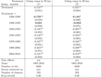
Table 5 shows the results for Gulag camps near a city. Gulag cities are different from the control group, and the difference (as measured by the coefficient before T reatment) is larger than for the war or evacuation. Gulag cities also grow significantly faster in 1926-1939. Negative coefficients of treatment-period interactions after 1959 are not large enough to compensate. In sum, having a Gulag camp nearby increases city growth by more than evacuation or being spared in the war. Figure 8 plots implied indices of city size for three treatment groups relative to the control group: occupied cities, cities that received evacuated enterprises, and cities with a Gulag camp within 50 km.

Dependent variable is an annualized growth rate of a city between two census years, %. Treatment Gulag camp in 50 km Gulag camp in 20 km

Indep. variable (1) (2)

Treatment 0.154** 0.255**

(0.051) (0.064)

Treatment×

1926-1939 0.170_** 0.145_*

(0.070) (0.089)

1939-1959 0.031 -0.053

(0.059) (0.075)

1959-1970 -0.195** -0.265**

(0.052) (0.065)

1970-1979 -0.148** -0.250**

(0.052) (0.065)

1979-1989 -0.167** -0.246**

(0.051) (0.064)

1989-2002 -0.204** -0.308**

(0.051) (0.064)

2002-2010 -0.121** -0.219**

(0.050) (0.063)

Year effects yes yes

Years 1987-2010 1987-2010

Number of obs 5636 5636

Errors clustered on city city

Number of clusters 763 763

R-sq overall 0.36 0.36

Robust SE in parentheses, ** - significant at 95% level, * - at 10% level.

Figure 8: City size index, as implied by separate panel estimations with city effects.

where to invest in infrastructure, drove both Gulag camp allocation and evacuations.These decisions also are correlated with the distance from the western border, and therefore with being close to the WWII front lines. There is no guarantee that random effects would be able to isolate the effects of war from the effect of Gulag, for example. To try to do so, I estimate a panel model with all three treatments included simultaneously. Table 6 and Figure 9 present the results.

Treatment Received Gulag Occupied evacuation in 50 km

Treatment -0.041 0.090 0.129**

(0.051) (0.057) (0.052) Treatment×

1926-1939 -0.161** -0.005 0.142_**

(0.069) (0.080) (0.069)

1939-1959 -0.054 0.049 0.013

(0.059) (0.067) (0.061) 1959-1970 0.141** -0.070 -0.154**

(0.054) (0.059) (0.054) 1970-1979 0.078 -0.095* -0.116

(0.053) (0.058) (0.053) 1979-1989 0.064 -0.079 -0.140**

(0.053) (0.058) (0.052) 1989-2002 0.122** -0.062 -0.169**

(0.053) (0.057) (0.052) 2002-1010 0.059 -0.075 -0.096* (0.051) (0.056) (0.051)

Year effects yes

Years 1897-2010

Number of obs 5636

Errors clustered on city

Number of clusters 763

R-sq overall 0.38

Dependent variable is an annualized growth rate of a city between two census years, in %. Robust SE in parentheses, ** - significant at 95% level, * - at 10% level.

Figure 9: City size index, as implied by a single panel model with city effects.

of a city (49% correlation), i.e. they are not actually random. To illustrate, Figure 10 plots the estimated random effects against geographical longitude.

Figure 10: Estimated city-level random effects and geographical longitude.

of Soviet policy. But a positive correlation with longitude is very nonintuitive. Eastern parts of Russia are famous for their cold climate, low population density, and remoteness. Large positive random effects for the majority of the eastern cities are unlikely to be the result of unobserved attractiveness of their locations; most likely they are the result of a general eastward bias in the Soviet location policy. That is, panel estimates are unable to distinguish between locations inherently attractive and locations favored by the Soviet policy.

In the next section, I employ an alternative approach. Instead of controlling for city heterogeneity with random effects, I explicitly control for the observable characteristics of a city. Among the control characteristics are geographical location, administrative status, past population level, and growth rate.

6

Matching Estimations

I analyze long-run trajectories of city growth using Abadie & Imbens (2002) bias-corrected matching estimator of average treatment effects for all three groups of factors: location relative to WWII front, industry evacuation, and Gulag. The choice of matching technique versus regression analysis allows me to remain agnostic about the functional form of the relationship between control variables and city growth. In principle, this relationship can be very unorthodox. The most obvious example of this is that the relationship between geographical variables and city growth does not have to be linear, or even have a simple functional form. Without a theory to guide the choice of a functional form, and with a large sample, matching estimators are a logical choice.

For each treated city, one or several matches from the control group are found. Matching cities must be as similar as possible to the treated city, with the similarity defined over the set of chosen characteristics. Then, the differences between treatment group and matching control group are analyzed in order to determine the effect of treatment.

similar administrative status and geographical location. As panel estimations show, the cities affected by WWII were different from the control group, even before the war. Therefore, I must also control for prior city growth and size. In all of the regressions, I exactly match cities on oblast center status. That is, I compare oblast centers with other oblast centers, and ordinary cities with other ordinary cities. Oblast centers may be more attractive than the average city because of their administrative functions.12

Cities also are matched on latitude, longitude, initial population level, and the rate of growth in the preceding time period. The algorithm looks for the closest matches in this four-dimensional space of matching characteristics (standardized by the sample variance), where the metric is given by the Euclidian distance (for details, see Abadie, Drukker, Herr & Imbens (2001)).

Finally, for each of the treatments, the cities are matched exactly on other treatments. For example, the growth of cities on both sides of WWII front lines is compared for those with the same evacuation status (whether enterprises were evacuated from the city, or to the city) and controlling for having a Gulag camp nearby. In the same way, cities that received evacuated plants are compared to cities that also were unaffected by WWII fighting, and to cities with the same Gulag status (presence or absence of a camp in the vicinity).

Table 7 presents the results for the WWII treatments. The effect of occupation is negative in 1939-1959 (as expected), but by 1970 the recovery is complete. There is no evidence that being occupied has any effect on city growth 25 years after the end of the war. This is in line with the results by Davis & Weinstein (2002), who found a similarly complete recovery from wartime destruction for Japanese cities.

12

Dependent variable isLnP opt−LnP opt₋1

(1) (2) (3)

Treatment variable 30 km to 200 km to

Occupied front front # of obs

Time period

1939-1959 -0.071** -0.074** -0.135** 624

(0.030) (0.030) (0.034)

1939-1970 -0.012 0.003 -0.063 625

(0.036) (0.037) (0.044)

1939-1979 0.038 0.040 -0.062 625

(0.042) (0.042) (0.051)

1939-1989 0.029 0.023 -0.070 629

(0.047) (0.048) (0.059)

1939-2002 0.074 0.013 -0.069 629

(0.051) (0.057) (0.065)

1939-2010 0.075 0.018 -0.068 627

(0.052) (0.062) (0.069)

% of obs treated 32 43 59

% of exact matches 84 86 85

Matching variables latitude, latitude, latitude,

population 1939, population 1939, population 1939, growth 1926-1939, growth 1926-1939, growth 1926-1939,

exact matching on oblast center oblast center oblast center

status, status, status,

evacuation (to, from), evacuation (to, from), evacuation(to, from), Gulag in 50 km. Gulag in 50 km. Gulag in 50 km.

Number of matches - 3, estimators are bias-adjusted for non-exact matching. Standard errors are heteroskedasticity- robust, ** denotes significance at 95% level, * - at 90% level.

As for evacuation status (Table 8), positive effects are observed for cities that received evacuation, but the effect is not statistically significant beyond 1970. Interestingly, the coef-ficient for treatment effect does not diminish over time, but its variance grows significantly. Perhaps to fully explore the heterogeneity in the impact of evacuation, the researchers would need to collect more detailed archival data on the number of evacuees, size, or specialization of the enterprises evacuated.

Restricting matching destination-cities to the cities in the same macro-region does not change the results (column (2)). Cities, where industrial establishments did not return after the war, grew slower than the average until 1959, but the effect is short-lived and disappears in 1970 and later (column (5)).

As in the panel estimations, the positive and long-lasting effects for cities that sent plants into evacuation (column (3)) are due to the same statistical artifact of Soviet regional prior-ities and selection. When the matching algorithm places too much weight on geographical proximity, I end up pairing industrial cities in central Russia, where enterprises were evac-uated from, with cities in the same region where there was no important industry. When I do not match by longitude, this effect disappears (column (4)).

In contrast, the presence of a Gulag camp has a long-lasting and positive impact on city growth (table 9, column (1)). The difference between treatment and control group does not diminish, it actually continues to grow, even up to the present time! City size indices for all three treatments are plotted on Figure 11.13

In columns (2)-(5), of Table 9, I report the estimates of the treatment effects for dif-ferent types of Gulag camps. Camps that specialized in agriculture/forestry (most of these were logging operations, where prisoners worked) or construction had relatively weaker effect on cities. In “agriculture/forestry” camps, prisoners were used mainly to extract valuable resource (timber), not to create infrastructure for future development. Among the

“con-13

Dependent variable is LnP opt−LnP opt₋1

(1) (2) (3) (4) (5)

Treatment variable enterprises enterprises enterprises enterprises enterprises

evacuated evacuated evacuated evacuated did not # of obs

to to from from return

Time period

1939-1959 0.109** 0.109** 0.378** -0.063* -0.106** 624 (0.036) (0.0367) (0.037) (0.038) (0.047)

1939-1970 0.120* 0.120* 0.262** -0.005 -0.051 625

(0.062) (0.062) (0.041) (0.043) (0.055)

1939-1979 0.114 0.113 0.188** 0.004 -0.056 625

(0.073) (0.073) (0.044) (0.046) (0.060)

1939-1989 0.122 0.120 0.246** -0.013 -0.041 629

(0.082) (0.082) (0.049) (0.050) (0.073)

1939-2002 0.117 0.117 0.173** -0.025 -0.041 629

(0.084) (0.084) (0.051) (0.053) (0.72)

1939-2010 0.101 0.099 0.137** 0.021 -0.038 627

(0.085) (0.085) (0.052) (0.101) (0.068)

% of obs treated 25 25 16 16 8

% of exact matches 99 62 63 63 63

Matching variables latitude, latitude, latitude, latitude, latitude, longitude, longitude, longitude,

population population population population population

1939, 1939, 1939, 1939, 1939,

growth growth growth growth growth 1926-1939, 1926-1939, 1926-1939, 1926-1939, 1926-1939,

exact matching on oblast oblast oblast oblast oblast center center center center center status, status, status, status, status, war front war front war front war front war front in 200 km, in 200 km, in 200 km, in 200 km, in 200 km,

Gulag in Gulag in Gulag in Gulag in Gulag in 50 km. 50 km, 50 km. 50 km, 50 km,

Urals, longitude. longitude. Siberia.

Number of matches - 3, estimators are bias-adjusted for non-exact matching. Standard errors are heteroskedasticity- robust, ** denotes significance at 95% level, * - at 90% level.

Dependent variable is LnP opt−LnP opt₋1

Gulag camp in 50 km

(1) (2) (3) (4) (5)

Treatment variable resource agriculture and

all camps extraction industry forestry construction # of obs

Time period

1926-1939 0.104** 0.126* 0.223** 0.134** 0.097** 459

(0.046) (0.076) (0.061) (0.057) (0.048)

1939-1959 0.076** 0.218** 0.161** 0.060 0.090** 458

(0.031) (0.053) (0.033) (0.048) (0.031)

1926-1959 0.177** 0.323** 0.381** 0.190** 0.185** 458

(0.061) (0.094) (0.074) (0.085) (0.062)

1926-1970 0.176** 0.279** 0.387** 0.162* 0.200** 458

(0.073) (0.085) (0.088) (0.085) (0.073)

1926-1979 0.198** 0.321** 0.416** 0.195** 0.224** 458

(0.082) (0.093) (0.099) (0.089) (0.084)

1926-1989 0.222** 0.381** 0.422** 0.213** 0.216** 459

(0.088) (0.089) (0.104) (0.092) (0.095)

1926-2002 0.217** 0.355* 0.412** 0.214** 0.215** 459

(0.091) (0.096) (0.109) (0.094) (0.095)

1926-2010 0.226** 0.398** 0.455** 0.273** 0.231** 458

(0.093) (0.095) (0.111) (0.099) (0.098)

% of obs treated 46 18 24 13 34

% of exact matches 97 91 95 93 97

Matching variables latitude, latitude, latitude, latitude, latitude, longitude longitude longitude longitude longitude population population population population population

1926, 1926, 1926, 1926, 1926,

growth growth growth growth growth

1897-1926, 1897-1926, 1897-1926, 1897-1926, 1897-1926,

exact matching on oblast oblast oblast oblast oblast

center center center center center

status, status, status, status, status, evacuation evacuation evacuation evacuation evacuation (to, from), (to, from), (to, from), (to, from), (to, from), war front war front war front war front war front in 30 km in 30 km in 30 km in 30 km in 30 km

Number of matches - 3, estimators are bias-adjusted for non-exact matching. Standard errors are heteroskedasticity- robust, ** denotes significance at 95% level, * - at 90% level.

struction” camps were those created for the infamous infrastructural projects of the 1930s: Northern Railroad, White-Sea-Baltic canal. Some of these projects proved a failure and were abandoned.

On the other hand, camps that specialized in industrial production (either primary in-dustries or other manufacturing) were creating this coveted “eastern industrial base” of the Soviet Union. Their impact on city size is twice as strong as that of an average camp.

Figure 11: City size index, as implied by matching estimations.

Table 10 presents estimated treatment effects for the different types of construction in Gulag. Consistent with Table 9, construction of industrial objects and housing leads to stronger long-run population increases. Construction of infrastructure shows weaker effects.

7

Conclusion

Dependent variable isLnP opt−LnP opt₋1

Gulag camp in 50 km

(1) (2) (3) (4)

Treatment variable industrial industrial

construction construction housing infrastructure

(primary) (manufacturing) construction construction # of obs

Time period

1926-1939 0.206** 0.097* 0.160** 0.105** 459

(0.062) (0.056) (0.067) (0.049)

1939-1959 0.248** 0.141** 0.146** 0.082** 458

(0.065) (0.036) (0.041) (0.031)

1926-1959 0.460** 0.236** 0.302** 0.184** 458

(0.093) (0.072) (0.086) (0.063)

1926-1970 0.399** 0.227* 0.290** 0.212** 458

(0.094) (0.079) (0.094) (0.076)

1926-1979 0.412** 0.255** 0.318** 0.243** 458

(0.109) (0.087) (0.102) (0.087)

1926-1989 0.393** 0.274** 0.333** 0.232** 459

(0.108) (0.092) (0.106) (0.095)

1926-2002 0.389** 0.282** 0.336** 0.226** 459

(0.115) (0.096) (0.109) (0.097)

1926-2010 0.443** 0.337** 0.392** 0.241*** 458

(0.120) (0.100) (0.117) (0.101)

% of obs treated 11 17 21 31

% of exact matches 90 95 94 97

Matching variables latitude, latitude, latitude, latitude, longitude longitude longitude longitude population population population population

1926, 1926, 1926, 1926,

growth growth growth growth

1897-1926, 1897-1926, 1897-1926, 1897-1926,

exact matching on oblast center oblast center oblast center oblast center

status, status, status, status,

evacuation evacuation evacuation evacuation (to, from), (to, from), (to, from), (to, from), war front war front war front war front in 30 km in 30 km in 30 km in 30 km

Number of matches - 3, estimators are bias-adjusted for non-exact matching. Standard errors are heteroskedasticity- robust, ** denotes significance at 95% level, * - at 90% level.

To what extent was Gulag responsible for the reallocation of productive resources toward the remote regions of the USSR? Millions of people went through the Gulag system, but compared to the Soviet population, the size of Gulag labor force does not not seem eco-nomically significant. Even at its maximum, the able-bodied population of Gulag did not exceed 2% of the Soviet labor force (Khlevnyuk (2004)). A vast majority of Gulag camps were located close to population centers, where the size of the local labor force significantly exceeded the size of the camp population. But the presence of a camp is a good indicator of a local deficit of labor. Gulag was not the only tool of Soviet regional industrial policy, but its presence is a good signal that the location was chosen by the Soviet authorities for investment projects. What we observe in the data is probably not the effect of Gulag per se, but rather the combined effect of Soviet location policy for which Gulag is a good proxy.

Gulag camps were heterogeneous. Some of the camp locations were oriented exclusively toward resource extraction, were not planned as permanent settlements, and quickly withered after Stalin’s death. We know examples of abandoned camps in the middle of empty frozen landscapes. But the camps that were located close to the existing population centers were used to build basic industrial and public infrastructure, and to supply labor for industrial facilities, a part of long-term regional planning strategies. Such locations continue to attract population even after the Gulag system (and prison labor in general) has stopped functioning as a source of slave labor.

as (and indeed were) permanent. My findings provide yet another illustration of “successful” regional policy. It a strong suggestion that to be able to change economic geography in the long run, the impact of regional policy has to be as significant as Stalin’s industrialization of the eastern USSR.

The strongest long-term effect found here is for Gulag camps that specialized in industry, industrial construction, and construction of housing. What are the mechanisms behind this? Do Stalin-era investments in capital and infrastructure still make the cities attractive, or are there other history-dependent factors? Is there a difference in local industrial structure between cities with Gulag camps and cities without them? What about sectoral diversity and specialization? Is there a difference in human capital? I leave these questions for further research.

References

Abadie, A., Drukker, D., Herr, J. L. & Imbens, G. W. (2001), ‘Implementing Matching Estimators for Average Treatment Effects in Stata’, The Stata Journal 1, 1–18.

Abadie, A. & Imbens, G. W. (2002), Simple and Bias-Corrected Matching Estimators for Average Treatment Effects, NBER Technical Working Papers 0283, National Bureau of Economic Research, Inc.

Andrienko, Y. & Guriev, S. M. (2004), ‘Determinants of Interregional Mobility in Russia’,

Economics of Transition 12(1), 1–27.

Andronikov, N. G., ed. (1975), Istoria Vtoroi Mirovoi Voiny 1939-1945 (History of WWII 1939-1945), Vol. 4, Voenizdat, Moscow.

Applebaum, A. (2003),GULAG: A History, Doubleday.

Bosker, M., Brakman, S., Garretsen, H. & Schramm, M. (2007), ‘Looking for Multiple Equilibria When Geography Matters: German City Growth and the WWII Shock’,

Journal of Urban Economics 61(1), 152–169.

Brakman, S., Garretsen, H. & Schramm, M. (2004), ‘The Strategic Bombing of German Cities during World War II and its Impact on City Growth’, Journal of Economic Geography 4(2), 201–218.

Davis, D. R. & Weinstein, D. E. (2008), ‘A Search for Multiple Equilibria in Urban Industrial Structure’, Journal of Regional Science48.

Dexter, K. & Rodionov, I. (2012), ‘The Factories, Research and Design Establishments of the Soviet Defence Industry: a Guide: Version 13’, University of Warwick, Department of Economics, http://warwick.ac.uk/vpk/.

Dienes, L. (1972), ‘Investment Priorities in Soviet Regions’, Annals of the Association of American Geographers 62(3), 437–454.

Dyker, D. A. (1983), The Process of Investment in the Soviet Union, Cambridge University Press, Cambridge, UK.

Gang, I. N. & Stuart, R. C. (1999), ‘Mobility Where Mobility is Illegal: Internal Migration and City Growth in the Soviet Union’,Journal of Population Economics12(1), 117–134. Harris, C. D. (1970), Population of Cities of the Soviet Union, 1897, 1926, 1939, 1959 and

1967 : with tables, maps, and gazetteer, American Geographical Society.

Harrison, M. (1988), ‘Resource Mobilization for World War II: the U.S.A., U.K., U.S.S.R., and Germany, 1938-1945’, Economic History Review41, 171–192.

Harrison, M. (1990), ‘Stalinist Industrialisation and the Test of War’, History Workshop Journal (29), 65–84.

Hooson, D. J. (1968), The Growth of Cities in Pre-Soviet Russia, in R. P. Beckinsale & J. M. Houston, eds, ‘Urbanization and its Problems: Essays in Honor of E. W. Gilbert’, Oxford: Basil Blackwell.

Huzinec, G. A. (1977), ‘Reexamination Of Soviet Industrial Location Theory’, The Profes-sional Geographer 29(3), 259–265.

Ivanova, G. M. (2006), Istoria Gulaga 1918-1958 / History of Gulag 1918-1958, Nauka, Moscow.

Iyer, S. D. (2003), ‘Increasing Unevenness in the Distribution of City Sizes in Post-Soviet Russia’, Eurasian Geography and Economics 44(5), 348–367.

Khlevnyuk, O. V., ed. (2004), Istoria Stalinskogo Gulaga / History of Stalin’s Gulag, Vol. 3 (Economika Gulaga / The Economy of Gulag), ROSSPEN.

Kozlov, M., ed. (1985), Velikaya Otechestvennaya Voina 1941-1945. Entsiklopediya. / The Great Patriotic War. An Encyclopedia., USSR Ministry of Defence, Institute of Military History and Sovetskaya Entsiklopediya, Moscow.

Kumo, K. (2006), Interregional Population Migration in Russia: Using an Origin-to-Destination Matrix, Discussion Paper Series a483, Institute of Economic Research, Hitotsubashi University.

Lieberman, S. R. (1983), ‘The Evacuation of Industry in the Soviet Union during World War II’, Soviet Studies 35, 90–102.

Miguel, E. & Roland, G. (2011), ‘The Long-run Impact of Bombing Vietnam’, Journal of Development Economics 96(1), 1–15.

Redding, S. J. & Sturm, D. M. (2008), ‘The Costs of Remoteness: Evidence from German Division and Reunification’, American Economic Review 98(5), 1766–97.

Redding, S. J., Sturm, D. M. & Wolf, N. (2011), ‘History and Industry Location: Evidence from German Airports’, The Review of Economics and Statistics93(3), 814–831. Rodgers, A. (1974), ‘The Locational Dynamics Of Soviet Industry’,Annals of the Association

of American Geographers 64(2), 226–240.