Munich Personal RePEc Archive
Selecting the Most Adequate Spatial
Weighting Matrix:A Study on Criteria
Herrera Gómez, Marcos and Mur Lacambra, Jesús and Ruiz
Marín, Manuel
July 2012
Selecting the Most Adequate Spatial Weighting Matrix:
A Study on Criteria
∗
Marcos Herrera (University of Zaragoza); [email protected]
Jesús Mur (University of Zaragoza); [email protected]
Manuel Ruiz (University of Murcia); [email protected]
Abstract
In spatial econometrics, it is customary to specify a weighting matrix, the so-called W matrix, by choosing one matrix from a finite set of matrices. The decision is extremely important because, if the W matrix is misspecified, the estimates are likely to be biased and inconsistent. However, the procedure to select W is not well defined and, usually, it reflects the judgments of the user. In this paper, we revise the literature looking for criteria to help with this problem. Also, a new nonparametric procedure is introduced. Our proposal is based on a measure of the information, conditional entropy. We compare these alternatives by means of a Monte Carlo experiment.
1
Introduction
The weighting matrix is a very characteristic element of spatial models and, frequently, is the cause of dispute in relation to what it is and how it should be specified. This matrix is a key element for modeling spatial data and it has received considerable attention (Anselin, 2002). However, from our point of view, we still do not have a complete convincing answer to both questions.
Formally, for any spatial sample, the spatial weights matrix is anN×N positive matrix, whereN
is the size of the data set:
∗Paper presented at the VIth World Conference - Spatial Econometrics Association. Salvador, Brazil. July 11-13,
2012.
1Corresponding author: Department of Economic Analysis, University of Zaragoza. Gran Via 2-4 (50005). Zaragoza
W =
0 w1,2 · · · w1,j · · · w1,N
w2,1 0 · · · w2,j · · · w2,N
..
. ... ... · · · ·
wi,1 wi,2 ... 0 · · · wi,N
..
. ... ... ... ... · · ·
wN,1 wN,2 ... wN,j ... 0 , (1)
where the elements wij are the spatial weights. The spatial weights wij are non-zero when i and j
are hypothesized to be neighbors, and zero otherwise. By convention, the self-neighbor relation is excluded, so the diagonal elements ofW,wii= 0.
As a extensively used criterion for choosing the weights wij is that of geographical proximity
or distance. But, but this is not necessarily true for all applications as evidenced by the principle of allotopy stated by Ancot et al. (1982): “often what happens in a region is related with other
phenomena located in distinct and remote parts of the space”. The problem of the identification what observations are neighbors and how to introduce them in the analysis is not a particular problem of spatial econometrics. Similar problems there are in time series although in this case we have some clear indications: you have to look to the past and take into account also the frequency of the data. However, the space is irregular and heterogeneous and the influences may be of any type across space. Nearness, as claimed by Tobler (1970) is just one possibility.
We agree with Haining (2003, p.74) in the sequence of actions: “The first step of quantifying the structure of spatial dependence in a data set is to define for any set of points or area objects the spatial relationships that exist between them”. This is what Anselin (1988, p. 16) designates “the need to determine which other units in the spatial system have an influence on the particular unit under consideration (. . . ) expressed in the topological notions of neighborhood and nearest neighbor”. This step is crucial, but how do we do? In some cases, we might have enough information to fully specify a weighting matrix. In other cases, this matrix will be no more than a mere hypothesis. In fact, from our experience, we suspect that the second situation is the most common among practitioners.
The uncertainty that dominates the specification of the weighting matrix results from a problem of underidentification that affects, in general, to the most part of spatial models. Paelinck (1979, p.20) admits that there is an identification problem in the interdependent specifications used to model spatial behaviors. In terms of Lesage and Pace (2009, p.8), an unrestricted spatial autoregressive process like the following:
yi=αijyj+αikyk+xiβ+εi
yj =αjiyi+αjkyk+xjβ+εj
yk=αkiyi+αkjyj+xkβ+εk
εi;εj;εk ∼N 0;σ2
, (2)
parameters”. This is the reason why we need a spatial weighting matrix. Folmer and Oud (2008) propose what they call a structural approach to the problem of specifying a weighting matrix; Paci and Usai (2009) advocate for the use of proxies for the existence of spillover effects, etc. There are other proposals in the literature trying to amend the paucity of information that involves this problem. However, these methods also have restrictions and limitations.
The question of specifying a matrix seems really complex, although the practitioners prefer simple solutions. By large, the dominant approach involves an exogenous treatment of the problem. Nearby or neighboring units are treated as contiguous in a square binary connectivity matrix as, for example, in the traditional physical adjacent criteria, the k-nearest neighbors or the great circle distance.
Afterward, the binary matrix can be normalized in some way (by rows, columns, according to the total sum). Other matrices are constructed using some given function of the geographical distance between the centroids of the spatial units; the inverse of the distance between the two points is a popular decision; then the matrix can be normalized. Geography may be replaced by another domain in order to obtain others measures of distance. Recently various endogenous procedures have appeared like the AMOEBA algorithm (Getis and Aldsdat, 2004, Aldsdat and Getis, 2006), theCCC method of Mur and Paelinck (2010) or the entropy-based approach of Fernandez et al (2009). Although the differences between them, the basic idea of these algorithms appeared in the works of Kooijman (1976) and Openshaw (1977): using the information contained in the raw data, or in the residuals of the model in order to estimate the weighting matrix. This can be done if we have a panel of spatial data like in Conley and Molinari (2007), Bhattacharjee and Jensen-Butler (2006) and Beenstock et al (2010) but it is not easy in the case of a single cross-section. Finally, there are different well-known approaches which combine strong a prioris about the channels of interaction with endogenous inferential algorithms (Bodson and Peters, 1975, Dacey, 1965).
Bavaud (1998, p.153), given this state of affairs, is clearly skeptical,“there is no such thing as “true”, “universal” spatial weights, optimal in all situations” and continues by stating that the weighting matrix “must reflect the properties of the particular phenomena, properties which are bound to differ from field to field”. This means that, in the end, the problem of selecting a weighting matrix is a problem of model selection. In fact, different weighting matrices result in different spatial lags of the endogenous or the exogenous variables included in the model. Different equations with different regressors mean a model selection problem, even when the weighting matrix appears in the error term. This is the direction that we want to explore in the present paper as an alternative way to deal with the uncertainty of specifying the spatial weighting matrix.
Section 2 continues with a revision of the techniques of model selection that seem to fit better into our problem. We present our own non-parametric procedure in Section 3. Section 4 discusses a large Monte Carlo experiment in which we compare the small sample behavior of the most promising techniques. Section 5 concludes summarizing the most interesting results of our work.
2
Selecting a Weighting Matrix
y= Γy+xβ+ε, (3) wherey andεare (n×1) vectors,xis a (n×k) matrix,β is a (k×1) vector of parameters and Γ is a (n×n) matrix of interaction coefficients. The model is underidentified and a common solution to achieve identification consists in introducing some structure in the matrix Γ. This means to impose restrictions on the spatial interaction coefficients as, for example: Γ =ρW, whereρis a parameter and W is a matrix of weights. The termyW =W ythat appears on the right hand side of the equation is
one spatial lag of the endogenous variable. It is worth highlighting a couple of questions:
(i) The weighting matrix can be constructed in different ways using different interaction hypothesis. Each hypothesis results in a different weighting matrix and in a different spatial lag. In conclusion, different weighting matrices means different models containing different variables.
(ii) There are general guidelines about specifying a weighting matrix. For example: nearness, accessibility, influence, etc. However, it will be difficult to say which of these general principles would be better. The problem is clearly dominated by uncertainty.
Corrado and Fingleton (2011) discuss the construction of a weighting matrix from a theoretical perspective (they are worried, for example, about the information that the weights of a weighting matrix should contain). We prefer to focus on the statistical treatment of such uncertainty.
Let us assume that we have a set of N linearly independent weighting matrices, Υ =
{W1;W2;. . .;WN}. Usually N corresponds to a small number of different competing matrices but
in some cases this number may be quite large, reflecting a situation of great uncertainty. For instance, each matrix generates a different spatial lag and a different spatial model. These matrices may be related by different restrictions, resulting in a series of nested models. If the matrices are not related, the sequence of spatial models will be non-nested.
Two weighting matrices may be nested, for example, in the cases of binary rook-type and queen-type movements: all the links of the first matrix are contained in the second matrix which include also some other non-zero links. Discriminating between these two matrices is not difficult using the techniques for selecting between nested models. For example, in a maximum-likelihood approach (we would need the assumption of normality) it may be enough with a likelihood ratio or a Lagrange Multiplier. The last one is very simple as can be seen in Appendix 1.
For the case of non-nested matrices, we might find several proposals in the literature. Anselin (1984) provides the appropriate Cox-statistic for the case of:
H0:y=ρ1W1y+x1β1+ε1
HA:y=ρ2W2y+x2β2+ε2
)
, (4)
that Leenders (2002) converts into the J-test using an augmented regression like the following:
y= (1−α) [ρ1W1y+x1β1] +α
h
ˆ
ρ2W2y+x2βˆ2
i
+ν, (5)
being ˆρ2and ˆβ2the corresponding maximum-likelihood estimates (ML from now on) of the respective
extended to the comparison of a null model againstN different models. Kelejian (2008) maintains the approach of Leenders in aSARAR framework, which requiresGM M estimators:
y = ρiWiy+xiβi+ui=Ziγi+ui, (6)
ui = λiMiui+vi,
with i = 1,2, ...., N, Zi = (Wiy, xi) and γi = (ρi, β) . The J-test for selecting a weighting matrix
corresponds to the case wherexi =x; Wi =Mi but Wi 6=Wj. In order to obtain the test, we need
the estimation of an augmented regression, similar to that of (5):
y(ˆλ) =S(ˆλ)η+ε, (7) where S(ˆλ) = hZ(ˆλ), Fi, Z(λ) = (I−λW)Z (the same for y(ˆλ)), being ˆλ the estimate of λ for
the model of the null. MoreoverF = [Z1γˆ1, Z2γˆ2, . . . , ZNγˆN, W1Z1ˆγ1, W2Z2γˆ2, . . . , WNZNγˆN]. The
equation of (7) can be estimated by 2SLS using a matrix of instruments: ˆS = hZˆ(ˆλ),Fˆi, where ˆ
F =P F (similar forZ(ˆλ)) withP =H(H′H)−1
H andH =
x, W x, W2x
. Under the null that, for example, model 0 is correct and the 2SLS estimate ofη is asymptotically normal:
ˆ
η∼N
η0;σǫ2
ˆ
S′Sˆ−1
, (8)
whereη0= [γ′; 0]. The J-test checks that the last 2N parameters of vectorη are zero. Define ˆδ=Aηˆ
whereAis a 2N×(k+ 1 + 2N) matrix corresponding to the null hypothesis: H0: Aη= 0, then the
J-test can be formulated as a Wald statistic:
ˆ
δ′Vˆ−1ˆδ∼χ2(2N), (9)
being ˆV the estimated sample covariance of ˆδ.
Burridge and Fingleton (2010) show that the asymptotic Chi-square distribution can be a poor approximation. They advocate for a bootstrap resampling procedure that appears to improve both the size and the power of the J-test. There, remains implementation problems related to the use of consistent estimates for the parameters of (6) in the corresponding augmented regression. Kelejian (2008) proposes to construct the test using GMM-type estimators and Burridge (2011) suggests a mixture between GMM and likelihood-based moment conditions which controls more effectively the size of the test. Piras and Lozano (2010) present new evidence on the use of the J-test that relates the power of the test to a wise selection of the instruments.
The problem of model selection has been often treated, very successfully, from a Bayesian perspective (Leamer, 1978); this also includes the case of selecting a weight matrix in a spatial model by Hepple (1985a, b). The Bayesian approach, although highly demanding in terms of information, is appealing and powerful (Lesage and Pace, 2009). The same as the J-test, the starting point is a finite set of alternative models,M = {M1;M2;. . .;MN}. The specification of each model coincides
the vector ofk parameters. Then, the joint probability of the set of N models, k parameters andn
observations corresponds to:
p(M, θ, y) =π(M)π(θ|M)L(y|θ, M), (10)
whereπ(M) refers to the priors of the models, usuallyπ(M) = 1/N;π(θ|M) reflects the priors of the vector of conditional parameters to the model andL(y|θ, M) is the likelihood of the data conditioned
on the parameters and models. Using the Bayes’ rule:
p(M, θ|y) = p(M, θ, y)
p(y) =
π(M)π(θ|M)L(y|θ, M)
p(y) . (11) The posterior probability of the models, conditioned to the data, results from the integration of (11) over the parameter vectorθ:
p(M|y) =
Z
p(M, θ|y)dθ. (12) This is the measure of probability needed in order to compare different weighting matrices. Lesage and Pace (2009) discuss the case of a GaussianSARmodel:
y=ρiWiy+Xiβi+εi
εi∼i.i.d.N(0;σ2ǫ) )
, (13)
The log-marginal likelihood of (10) is:
p(M|y) =
Z
πβ β|σ2πσ σ2πρ(ρ)L(y|θ, M)dβdσ2dρ. (14)
They assume independence between the priors assigned to β and σ2, Normal-Inverse-Gamma
conjugate priors, and that forρ, aBeta(d, d) distribution. The calculations are not simple and, finally, “we must rely on univariate numerical integration over the parameterρto convert this(expression 14)
to the scalar expression necessary to calculatep(M|Y)needed for model comparison purposes” (Lesage and Pace, 2009, p 172). TheSEM case is solved in Lesage and Parent (2007); to our knowledge, the
SARARmodel of (6) remains still unsolved.
Model selection techniques may also have a role in this problem, specially if we have any preference for any weighting matrix. In other words, we are not considering the idea of a null hypothesis. There is a huge literature on model selection for nested and non-nested models with different purposes and criteria. In our case, we are looking for the most appropriate weighting matrix for the data. We consider that the Kullback-Leibler information criterion might be a good measure. Apart from Kullback-Leibler criterion, we can use the Akaike information criterion which is simple to obtain. This criterion assures a balance between fit and parsimony (Akaike, 1974). The expression of Akaike criterion is very well-known:
AICi=−2L
ˆ
being Lθˆ;y the log-likelihood of the model at the maximum-likelihood estimates, ˆθ, and q(k) a
penalty function that depends on the number of unknown parameters. Usually, the penalty function is simply equal toq(k) = 2k. The decision rule is to select the model, weighting matrix in our case, that produces the lowestAIC.
Recently Hansen (2007) introduced another perspective to the problem of model selection, which tries to reflect the confidence of the practitioner in the different alternatives. In general, the selection criteria that minimize the mean-square estimation error achieve a good balance between bias, due to misspecification errors, and variance due to parameter estimation. The optimal criterion would select the estimator with the lowest risk. This is what happens with the Bayesian concept of posterior probability, which combines prior with sampling information to select the best model; also with the selection criteria as, for example, the AIC or the SBIC statistics. The procedure of the J-test is a classical decision problem solved using only sampling information, with the purpose of minimizing the type II error and assuring a given type I error.
Expressed in another way, given our collection of weighting matricesW ={W1;W2;. . .;WN}, all
of which are referred to the same spatial model, the purpose is to select the matrixWn. This matrix
combines with the other terms of the model produces a vector of estimates, ˆθn(Wn), which minimizes
the risk. Hansen (2007) shows that further reductions in the mean-squared error can be attained by averaging across estimators. The averaging estimator forθis:
ˆ
θ(W) =
N X
n=1
̟nθˆn(Wn). (16)
As stated by Hansen and Racine (2010), the collection of weights, {̟n;n= 1,2, ..., N}should be
non-negative and linked on the unit simplex ofRN; N X
n=1
̟n= 1.
Subsequently, these weights̟n can be used to compare the adjustment of each model (W matrix)
with respect to the data.
3
A Non-Parametric Proposal for Selecting a Weighting
Matrix
This section presents a new non-parametric procedure for selecting a weighting matrix. The selection criterion is based on the idea that the most adequate matrix should produce more information with respect to the variables that we are trying to relate. The measure of information is a reformulation of the traditional entropy index in terms of what is calledsymbolic entropy, and it does not depend on
judgments of the user.
As explained in Matilla and Ruiz (2008), the procedure implies, first, transforming the series into a sequence of symbols which should capture all of the relevant information. Then we translate the inference to the space of symbols using appropriate techniques.
Beginning with the symbolization process, assuming that {xs}s∈S and {ys}s∈S are two spatial
processes, whereS is a set of locations in space. Denoted by Γl={σ1, σ2, . . . , σl}the set of symbols
f :{xs}s∈S →Γl, (17)
such that each elementxs is associated to a single symbolf(xs) =σis withis∈ {1,2, . . . , l}. We say
that locations∈S is of theσi−type, relative to the series {xs}s∈S, if and only if f(xs) =σis. We
callf thesymbolization map. The same procedure can be followed for a second series{ys}s∈S.
Denoted by{Zs}s∈S a bivariate process as:
Zs={xs, ys}. (18)
For this case, we define the set of symbols Ωlas the direct product of the two sets Γl, that is, Ω2l = Γl×Γl
whose elements are the formηij = σix, σ y j
. The symbolization function of the bivariate process would
be
g:{Zs}s∈S →Ω
2
l = Γl×Γl, (19)
defined by
g(Zs= (xs, ys)) = (f(xs), f(ys)) =ηij = σxi, σ y j
. (20)
We say thatsisηij−typeforZ= (x, y) if and only ifsisσix−typeforxandσ y
j −typefory.
In the following, we are going to use a simple symbolization functionf . Let Mx
e be the median of
the univariate spatial process{xs}s∈S and define an indicator function
τs= (
1 if xs≥Mex
0 otherwise . (21)
Letm≥2 be theembedding dimension; this is a parameter defined by the practitioner. For each
s∈S, letNsbe the set formed by the (m−1) neighbours ofs. We use the termm−surroundingto
denote the set formed by eachsandNs, such thatm−surroundingofxm(s) = xs, xs1, . . . , xsm−1
.
Let us define another indicator function for eachsi∈Ns:
ιssi =
(
0 if τs6=τsi
1 otherwise . (22)
Finally, we have a symbolization map for the spatial process{xs}s∈S asf :{xs}s∈S →Γm:
f(xs) = m−1
X
i=1
ιssi, (23)
where Γm={0,1, . . . , m−1}. The cardinality of Γmis equal tom.
Let us introduce some fundamental definitions:
Definition 1: The Shannon entropy, h(x), of a discrete random variable x is: h(x) = −
n P
i=1
p(xi)ln(p(xi)).
Definition 2: The entropyh(x, y) of a pair of discrete random variables (x, y) with joint distribution
p(x, y) is: h(x, y) =−P x
P
y
Definition 3: Conditional entropy h(x|y) with distribution p(x, y) is defined as: h(x|y) = −P
x P
y
p(x, y)ln(p(x|y)).
The last index,h(x|y), is the entropy of xthat remains wheny has been observed.
These entropy measures can be easily adapted to the empirical distribution of the symbols. Once the series have been symbolized, for a embedding dimensionm≥2, we can calculate the absolute and relative frequency of the collections of symbolsσx
is ∈Γl andσ
y js∈Γl.
The absolute frequency of symbolσx i is:
nσx
i = #{s∈S|s is σ
x
i −type f or x}. (24)
Similarly, for series{ys}s∈S, the absolute frequency of symbolσ y j is:
nσy j = #
s∈S|s is σjy−type f or y . (25)
Next, the relative frequencies can also be estimated:
p(σix)≡pσx i =
#{s∈S|s is σx
i −type f or x}
|S| =
nσx i
|S|, (26)
p σjy
≡pσy j =
#
s∈S|s is σyj −type f or y
|S| =
nσy j
|S|, (27)
where|S|denotes the cardinal of set S; in general|S|=N. Similarly, we calculate the relative frequency forηij∈Ω2l:
p(ηij)≡pηij =
#{s∈S|s is ηij−type}
|S| =
nηij
|S|. (28)
Finally, thesymbolic entropy for thetwo−dimensionalspatial series{Zs}s∈S is:
hZ(m) =− X
η∈Ω2
m
p(η)ln(p(η)). (29)
We can obtain the marginal symbolic entropies as
hx(m) =− X
σx∈Γm
p(σx)ln(p(σx)), (30)
hy(m) =− X
σy∈Γm
p(σy)ln(p(σy)). (31)
In turn(tern), we can obtain the symbolic entropy of y, conditioned by the occurrence of symbol σxin xas:
hy|σx(m) =−
X
σy∈Γm
We can also estimate the conditional symbolic entropy ofysgivenxs:
hy|x(m) = X
σx∈Γm
p(σx)h
y|σx(m). (33)
Let us move to the problem of choosing a weighting matrix for the relationship between the variables
xandy. This selection will be made from among a finite set of relevant weighting matrices. Denoted byW(x, y) ={W|∈ J } this set of matrices, whereJ is a set of index. We refer toW(x, y) as the
spatial-dependence structure set betweenxandy.
Denoted byK a subset of Γm, the space of symbols, and letW ∈ W(x, y) be a member of the set
of matrices. We can define
Kx
W ={σx∈ K|σxis admissible forW x}, (34)
whereadmissible indicates that the probability of symbol occurrence is positive. By Γx
m we denote the set of symbols which are admissible for{xs}s∈S. LetW0 ∈ W(x, y) be the
most informative weighting matrix for the relationship between x and y. Given the spatial process
{ys}s∈S, there is a subset K ⊆ Γm such that p KxW0|σ
y
> p(K∗x
W|σy) for all K∗ ⊆ Γm, W ∈
W(x, y)\ {W0} andσy∈Γym. Then
hW0x|y(m) = −
X
σy∈Γy
p(σy)
X
σx∈Kx Wo
p(σx|σy) ln (p(σx|σy))
(35)
≤ − X
σy∈Γy
pσy
X
σx∈K∗x W
p(σx|σy) ln (p(σx|σy))
=hW x|y(m).
In this way, we have proved the following theorem.
Theorem 1: Let {xs}
s∈S and {ys}s∈S two spatial processes. For a fixed embedding dimension
m≥2, withm∈N, if the most important weighting matrix that reveals the spatial-dependence
structure between xandy isW0∈ W(x, y)then
hW0x|y(m) = min
W∈W(x,y)
hW x|y(m) . (36)
Given the Theorem 1 and using the following property: hW x|y ≤ hW x, we propose the following
criterion for selecting between different matrices:
pseudo−R2= 1−hW x|y(m)/hW x(m).
4
The Monte Carlo Experiment
In this section, we generate a large number of samples from different data generation process (D.G.P.) to study the performance of different proposals: J-test, Bayesian approach, averaging estimator (Racine-Hansen) and conditional symbolic entropy.
Our major interest is to detect the weighting matrix more informative between different alternatives. For this, we have an unique explanatory variablex, the same in all models. But the D.G.P. uses different spatial structures, that isW =Wi, whereiis the matrix for thei−thalternative model.
Each experiment starts by obtaining a random map in a hypothetical two-dimensional space. This irregular map is reflected on the corresponding normalizedW matrix. In the first case, W is based on a matrix of 1s and 0s denoting contiguous and non-contiguous regions, respectively. Afterward, we normalize theW matrix so that the sum of each row is equal to 1.
The following global parameters are involved in theD.G.P.:
N ∈ {100,400,700,1000}, k∈ {4,5,7}, (37) where N is the sample size and k is the number of neighbors for each observation. The number of replications is equal 1000.
In the cases of nested models, we use the following matrices:
• W4= 4−nearest−neighbors
• W5= 5−nearest−neighbors
• W7= 7−nearest−neighbors
whereW7 containsW5 matrix andW5containsW4 matrix, before the standardization.
In the cases of non-nested models, all spatial weighting matrices contain 4 neighbors but we modify the criterion of neighborhood. In all cases, we assume the following non-nested matrices:
• W(1)= 4−nearest−neighbors
• W(2)= 5o−to−8o−nearest−neighbors
• W(1−2)= 1o−2o−5o−6o−nearest−neighbors
In this experiment, we want to simulate both linear and non-linear relationships between the variables
xandy.
In the first case, linearity, we control the relationship between variables using theexpected coefficient of determination(R2
y/x) based on a specification like this:
y=βx+θW x+ε. (38) Under equation (38), the expected coefficient of determination between the variables is equal to (assuming an unit variance ofxand inεas well as incorrelation between the two variables):
R2
y/x=
β2+ θ2
/m−1
β2+ θ2
We have considered different values for this coefficient:
R2y/x∈ {0.4; 0.6; 0.8} (39) For simplicity, in all cases we maintainβ = 0.5. The spatial lag parameter of x,θ, is obtained by deduction: θ=q(1−m)(β2(1−R2)−R2)
1−R2 .
Having defined the values of the parameters involved in the simulation, we can present the different processes used in the analysis.
DGP1: Linear
y=βx+θW x+ε (40)
DGP2: Non-linear 1
y= exph(βx+θW x+ε)1.25i
(41)
DGP3: Non-linear 2
y=1/(βx+θW x+ε)2 (42) In all cases: x∼ N(0,1), ε∼ N(0,1) and Cov(x, ε) = 0.
Results
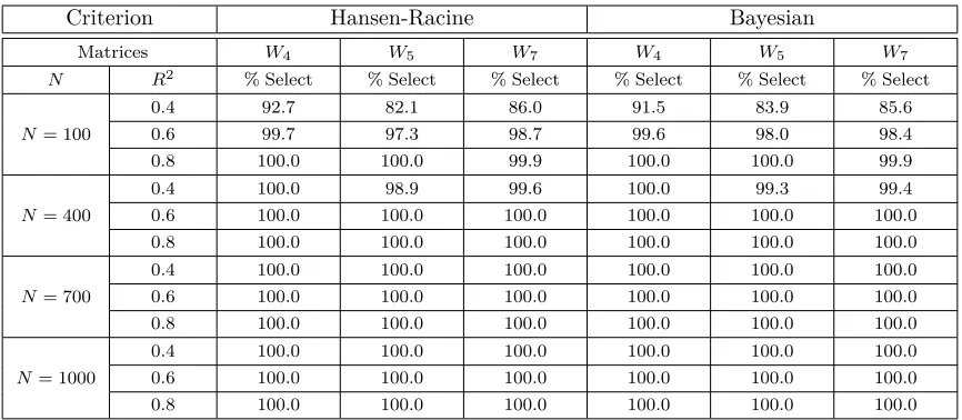
[image:13.612.90.523.503.692.2]The performance of Hansen-Racine, Bayesian, J-test and LM for the nested models are presented in Tables 1-9 . When the process is linear, Table 1, the selection made by criteria of Hansen-Racine and Bayesian is near to 100%, in almost all situations. The behavior of J-test and LM is similar, with results that exceed 85% of correct selection in almost all cases (Table 2). The LM is slightly higher for the case ofW7.
Table 1: DGP1: Linear Process. Nested Models
Criterion Hansen-Racine Bayesian
Matrices W4 W5 W7 W4 W5 W7
N R2 % Select % Select % Select % Select % Select % Select
0.4 92.7 82.1 86.0 91.5 83.9 85.6
N= 100 0.6 99.7 97.3 98.7 99.6 98.0 98.4
0.8 100.0 100.0 99.9 100.0 100.0 99.9
0.4 100.0 98.9 99.6 100.0 99.3 99.4
N= 400 0.6 100.0 100.0 100.0 100.0 100.0 100.0
0.8 100.0 100.0 100.0 100.0 100.0 100.0
0.4 100.0 100.0 100.0 100.0 100.0 100.0 N= 700 0.6 100.0 100.0 100.0 100.0 100.0 100.0
0.8 100.0 100.0 100.0 100.0 100.0 100.0
0.4 100.0 100.0 100.0 100.0 100.0 100.0 N= 1000 0.6 100.0 100.0 100.0 100.0 100.0 100.0
0.8 100.0 100.0 100.0 100.0 100.0 100.0
Table 2: DGP1: Linear Process. Nested Models
Criterion J-test LM
Matrices W4 W5 W7 W4 W5 W7
N R2 % Select % Select % Select % Select % Select % Select
0.4 71.2 53.1 55.8 89.7 73.3 60.9
N= 100 0.6 89.5 86.5 87.1 90.3 91.0 97.3
0.8 87.4 85.6 88.1 88.0 90.5 99.9
0.4 89.5 88.7 88.5 90.4 92.3 99.9
N= 400 0.6 87.8 85.3 87.7 88.7 91.5 100.0
0.8 89.9 86.2 88.0 91.0 90.4 100.0
0.4 87.4 87.4 89.2 88.8 93.7 100.0
N= 700 0.6 89.1 85.2 87.1 89.4 91.7 100.0
0.8 91.0 86.8 87.4 91.8 92.7 100.0
0.4 88.4 86.6 89.5 89.1 92.2 100.0
N= 1000 0.6 90.6 87.8 90.5 91.7 93.1 100.0
0.8 87.8 86.2 89.6 89.1 91.9 100.0
Note: % Select is the number of times that eachW is selected correctly. Replications: 1000.
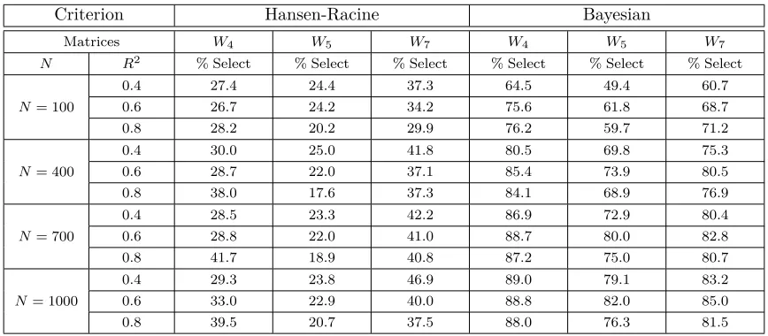
When the generating process is non-linear, DGP2, the results are significantly altered. The Bayesian approach is the best performance with a maximum value of 89% of correct selection when the sample size is equal to 1000. The LM test tends to select subidentified matrices and due to this we observe high rates of selection forW4. In this case, R2’s are presented only to identify the value
involved in the generation ofθ.
Table 3: DGP2: Non-Linear Process 1. Nested Models
Criterion Hansen-Racine Bayesian
Matrices W4 W5 W7 W4 W5 W7
N R2 % Select % Select % Select % Select % Select % Select
0.4 27.4 24.4 37.3 64.5 49.4 60.7
N= 100 0.6 26.7 24.2 34.2 75.6 61.8 68.7
0.8 28.2 20.2 29.9 76.2 59.7 71.2
0.4 30.0 25.0 41.8 80.5 69.8 75.3
N= 400 0.6 28.7 22.0 37.1 85.4 73.9 80.5
0.8 38.0 17.6 37.3 84.1 68.9 76.9
0.4 28.5 23.3 42.2 86.9 72.9 80.4
N= 700 0.6 28.8 22.0 41.0 88.7 80.0 82.8
0.8 41.7 18.9 40.8 87.2 75.0 80.7
0.4 29.3 23.8 46.9 89.0 79.1 83.2
N= 1000 0.6 33.0 22.9 40.0 88.8 82.0 85.0
0.8 39.5 20.7 37.5 88.0 76.3 81.5
[image:14.612.89.523.430.620.2]Table 4: DGP2: Non-Linear Process 1. Nested Models
Criterion J-test LM
Matrices W4 W5 W7 W4 W5 W7
N R2 % Select % Select % Select % Select % Select % Select
0.4 14.9 4.5 10.3 88.6 21.8 12.7
N= 100 0.6 28.4 13.2 18.3 88.1 35.2 23.1
0.8 28.7 12.7 20.0 91.1 32.1 24.8
0.4 42.3 26.8 34.4 89.5 50.4 38.7
N= 400 0.6 53.8 33.7 42.9 89.1 53.7 46.5
0.8 48.1 28.0 35.3 91.0 50.6 39.3
0.4 58.2 35.3 43.4 90.3 55.7 47.7
N= 700 0.6 61.7 45.9 53.1 90.5 63.9 58.4
0.8 54.1 33.8 42.3 88.7 57.7 47.1
0.4 66.4 50.1 51.4 91.1 65.4 58.0
N= 1000 0.6 67.6 52.2 58.8 89.2 68.5 62.2
0.8 60.5 39.0 47.0 88.6 56.1 52.2
Note: % Select is the number of times that eachW is selected correctly. Replications: 1000.
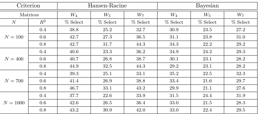
[image:15.612.92.522.411.601.2]When the non-linearity is incremented, DGP3, there is no criterion that provides adequate information about the genuine generating process. In this case, we can observe how the LM test tends to select the matrix with the least neighbors in all cases.
Table 5: DGP3: Non-Linear Process 2. Nested Models
Criterion Hansen-Racine Bayesian
Matrices W4 W5 W7 W4 W5 W7
N R2 % Select % Select % Select % Select % Select % Select
0.4 38.8 25.2 32.7 30.9 23.5 27.2
N= 100 0.6 42.7 27.3 36.5 31.1 23.8 31.0
0.8 42.7 31.7 44.3 34.3 22.2 29.2
0.4 40.6 23.3 36.2 34.9 24.2 29.3
N= 400 0.6 40.7 26.8 38.7 30.1 23.1 28.2
0.8 44.9 32.5 44.3 29.2 23.1 28.2
0.4 39.3 25.1 33.1 35.2 22.5 32.3
N= 700 0.6 41.4 26.9 38.8 33.4 21.6 29.7
0.8 46.7 33.1 43.2 29.9 21.1 27.6
0.4 37.7 22.6 33.9 31.5 24.4 31.9
N= 1000 0.6 42.6 26.5 36.4 33.0 21.5 28.3
0.8 43.2 30.9 42.0 33.0 22.4 29.5
Table 6: DGP3: Non-Linear Process 2. Nested Models
Criterion J-test LM
Matrices W4 W5 W7 W4 W5 W7
N R2 % Select % Select % Select % Select % Select % Select
0.4 0.3 0.4 0.2 89.4 5.5 0.6
N= 100 0.6 0.5 0.0 0.6 90.6 5.3 1.6
0.8 0.4 0.0 0.5 90.0 3.3 0.9
0.4 0.4 0.0 0.2 89.9 5.1 0.3
N= 400 0.6 0.3 0.1 0.3 89.1 4.3 0.9
0.8 0.2 0.0 0.1 90.8 3.5 0.3
0.4 0.4 0.2 0.4 90.7 5.1 1.0
N= 700 0.6 0.1 0.0 0.0 90.4 4.7 1.0
0.8 0.1 0.0 0.3 90.3 4.7 0.9
0.4 0.7 0.0 0.4 88.6 4.0 1.2
N= 1000 0.6 0.4 0.0 0.0 89.0 5.0 0.3
0.8 0.4 0.1 0.3 89.7 3.2 0.7
Note: % Select is the number of times that eachW is selected correctly. Replications: 1000.
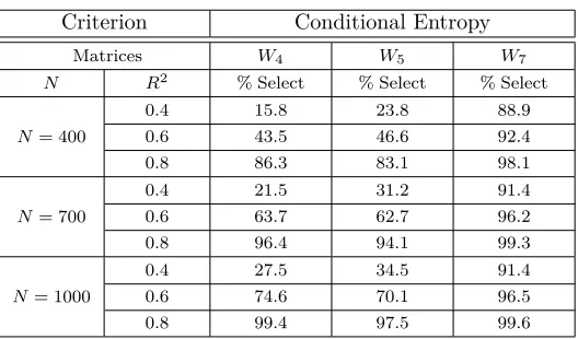
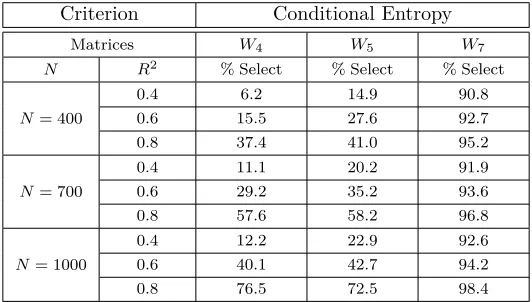
The behavior of the Conditional Entropy is presented in the Tables 7-9. We apply the following rule to select the embedding dimensionm: m2·5≈N. That is, on average, each symbol should have
an expected frequency closed to 5. Therefore, we use for nested modelsm = 8 for all cases because
containW7,W5 andW4. Due to this rule, the minimum sample size is 400.
For the linear process, Table 7, Entropy does not make a good selection in comparison to the other criteria.
Table 7: DGP1: Linear Process. Nested Models
Criterion Conditional Entropy
Matrices W4 W5 W7
N R2 % Select % Select % Select
0.4 15.8 23.8 88.9
N= 400 0.6 43.5 46.6 92.4
0.8 86.3 83.1 98.1
0.4 21.5 31.2 91.4
N= 700 0.6 63.7 62.7 96.2
0.8 96.4 94.1 99.3
0.4 27.5 34.5 91.4
N= 1000 0.6 74.6 70.1 96.5
0.8 99.4 97.5 99.6
Note: % Select is the number of times that eachW is selected correctly. Replications: 1000.
For the non-linear process 1, DGP2, the performance of Conditional Entropy improves and it reachs values over 90% in several cases. The behavior is similar to the Bayesian criterion, except for
R2 = 0.4. In the case of DGP3, the percentage of correct selection of the matrix is higher than the
[image:16.612.175.439.453.608.2]Table 8: DGP2: Non-Linear Process 1. Nested Models
Criterion Conditional Entropy
Matrices W4 W5 W7
N R2 % Select % Select % Select
0.4 16.8 23.8 88.3
N= 400 0.6 45.2 46.6 92.6
0.8 87.2 83.1 98.2
0.4 23.4 31.2 88.9
N= 700 0.6 59.1 62.7 96.4
0.8 96.6 94.1 99.8
0.4 32.8 34.5 91.4
N= 1000 0.6 73.3 70.1 96.5
0.8 98.7 97.5 99.6
[image:17.612.173.439.342.493.2]Note: % Select is the number of times that eachW is selected correctly. Replications: 1000.
Table 9: DGP3: Non-Linear Process 2. Nested Models
Criterion Conditional Entropy
Matrices W4 W5 W7
N R2 % Select % Select % Select
0.4 6.2 14.9 90.8
N= 400 0.6 15.5 27.6 92.7
0.8 37.4 41.0 95.2
0.4 11.1 20.2 91.9
N= 700 0.6 29.2 35.2 93.6
0.8 57.6 58.2 96.8
0.4 12.2 22.9 92.6
N= 1000 0.6 40.1 42.7 94.2
0.8 76.5 72.5 98.4
Note: % Select is the number of times that eachW is selected correctly. Replications: 1000.
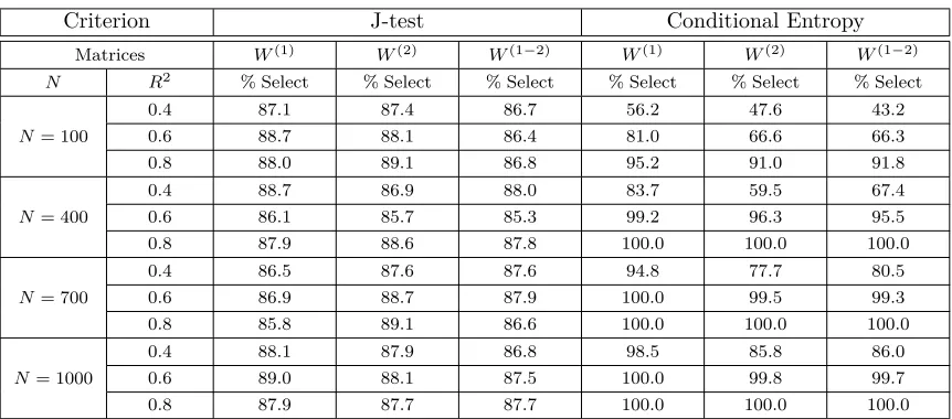
In the following Tables 10-15, we present the results for non nested models. In similar way as in nested models, when the process is linear,DGP1, the percentage of correct selection of Hansen-Racine criterion and Bayesian approach is almost of 100%. The behavior of J-test is stable at around 88% of correct selection. With regard to Conditional Entropy, its performance improves when theR2and
Table 10: DGP1: Linear Process. Non-Nested Models
Criterion Hansen-Racine Bayesian
Matrices W(1) W(2) W(1−2) W(1) W(2) W(1−2)
N R2 % Select % Select % Select % Select % Select % Select
0.4 99.6 99.4 99.8 99.6 99.5 99.8
N= 100 0.6 100.0 100.0 100.0 100.0 100.0 100.0
0.8 100.0 100.0 100.0 100.0 100.0 100.0
0.4 100.0 100.0 100.0 100.0 100.0 100.0 N= 400 0.6 100.0 100.0 100.0 100.0 100.0 100.0
0.8 100.0 100.0 100.0 100.0 100.0 100.0
0.4 100.0 100.0 100.0 100.0 100.0 100.0 N= 700 0.6 100.0 100.0 100.0 100.0 100.0 100.0
0.8 100.0 100.0 100.0 100.0 100.0 100.0
0.4 100.0 100.0 100.0 100.0 100.0 100.0 N= 1000 0.6 100.0 100.0 100.0 100.0 100.0 100.0
0.8 100.0 100.0 100.0 100.0 100.0 100.0
Note: % Select is the number of times that eachW is selected correctly. Replications: 1000.
Table 11: DGP1:Linear Process. Non-Nested Models
Criterion J-test Conditional Entropy
Matrices W(1) W(2) W(1−2) W(1) W(2) W(1−2)
N R2 % Select % Select % Select % Select % Select % Select
0.4 87.1 87.4 86.7 56.2 47.6 43.2
N= 100 0.6 88.7 88.1 86.4 81.0 66.6 66.3
0.8 88.0 89.1 86.8 95.2 91.0 91.8
0.4 88.7 86.9 88.0 83.7 59.5 67.4
N= 400 0.6 86.1 85.7 85.3 99.2 96.3 95.5
0.8 87.9 88.6 87.8 100.0 100.0 100.0
0.4 86.5 87.6 87.6 94.8 77.7 80.5
N= 700 0.6 86.9 88.7 87.9 100.0 99.5 99.3
0.8 85.8 89.1 86.6 100.0 100.0 100.0
0.4 88.1 87.9 86.8 98.5 85.8 86.0
N= 1000 0.6 89.0 88.1 87.5 100.0 99.8 99.7
0.8 87.9 87.7 87.7 100.0 100.0 100.0
Note: % Select is the number of times that eachW is selected correctly. Replications: 1000.
[image:18.612.91.522.364.554.2]Table 12: DGP2: Non-Linear Process 1. Non-Nested Models
Criterion Hansen-Racine Bayesian
Matrices W(1) W(2) W(1−2) W(1) W(2) W(1−2)
N R2 % Select % Select % Select % Select % Select % Select
0.4 14.6 13.4 26.9 81.8 84.8 79.8
N= 100 0.6 13.6 12.8 26.3 93.1 91.6 91.0
0.8 21.3 22.8 27.8 95.0 94.7 95.0
0.4 14.6 14.7 26.1 95.0 96.1 95.6
N= 400 0.6 19.3 17.4 27.4 97.9 98.5 97.2
0.8 28.7 27.8 31.2 98.0 97.4 97.5
0.4 16.8 13.9 26.2 97.5 97.1 97.0
N= 700 0.6 20.7 22.7 24.1 98.5 98.3 98.8
0.8 32.8 31.7 28.8 98.3 98.3 99.9
0.4 15.5 15.5 21.9 98.8 98.5 97.9
N= 1000 0.6 21.2 23.4 28.8 99.1 99.3 99.0
0.8 35.4 34.3 33.3 99.3 99.0 99.0
Note: % Select is the number of times that eachW is selected correctly. Replications: 1000.
Table 13: DGP2:Non-Linear Process 1. Non-Nested Models
Criterion J-test Conditional Entropy
Matrices W(1) W(2) W(1−2) W(1) W(2) W(1−2)
N R2 % Select % Select % Select % Select % Select % Select
0.4 51.1 50.2 47.3 56.2 38.6 43.2
N= 100 0.6 70.9 68.0 67.5 81.0 66.7 66.3
0.8 71.6 73.6 73.4 95.2 91.2 91.8
0.4 80.0 79.9 77.7 85.4 59.5 68.1
N= 400 0.6 83.3 83.3 81.6 99.3 96.3 95.5
0.8 84.0 85.2 83.2 100.0 100.0 100.0
0.4 80.9 85.0 80.9 96.0 75.8 79.0
N= 700 0.6 84.1 86.0 83.3 100.0 99.2 98.7
0.8 84.6 86.2 86.0 100.0 100.0 100.0
0.4 86.3 83.5 83.6 98.5 86.8 86.7
N= 1000 0.6 85.2 85.9 83.9 100.0 99.8 99.7
0.8 85.3 86.0 84.7 100.0 100.0 100.0
Note: % Select is the number of times that eachW is selected correctly. Replications: 1000.
[image:19.612.92.522.364.554.2]Table 14: DGP3: Non-Linear Process 2. Non-Nested Models
Criterion Hansen-Racine Bayesian
Matrices W(1) W(2) W(1−2) W(1) W(2) W(1−2)
N R2 % Select % Select % Select % Select % Select % Select
0.4 35.7 34.3 37.0 30.3 30.0 29.9
N= 100 0.6 40.0 39.9 41.8 27.9 31.6 27.2
0.8 46.1 44.9 43.9 21.8 24.2 22.7
0.4 34.8 32.5 36.1 26.1 27.1 28.2
N= 400 0.6 42.2 42.1 41.3 27.5 28.4 29.3
0.8 48.7 49.0 47.6 24.1 22.8 23.7
0.4 34.6 34.4 34.8 27.7 28.2 30.8
N= 700 0.6 41.5 39.6 40.9 27.4 28.0 30.7
0.8 48.0 47.1 46.3 22.5 23.1 20.9
0.4 35.9 36.2 35.8 28.6 30.8 26.6
N= 1000 0.6 43.5 41.1 41.6 27.9 27.3 27.9
0.8 50.3 48.0 47.3 21.3 22.7 23.2
Note: % Select is the number of times that eachW is selected correctly. Replications: 1000.
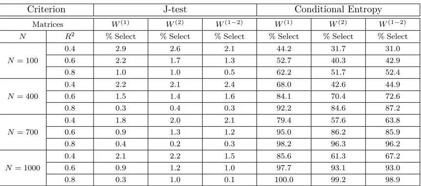
Table 15: DGP3: Non-Linear Process 2. Non-Nested Models
Criterion J-test Conditional Entropy
Matrices W(1) W(2) W(1−2) W(1) W(2) W(1−2)
N R2 % Select % Select % Select % Select % Select % Select
0.4 2.9 2.6 2.1 44.2 31.7 31.0
N= 100 0.6 2.2 1.7 1.3 52.7 40.3 42.9
0.8 1.0 1.0 0.5 62.2 51.7 52.4
0.4 2.2 2.1 2.4 68.0 42.6 44.9
N= 400 0.6 1.5 1.4 1.6 84.1 70.4 72.6
0.8 0.3 0.4 0.3 92.2 84.6 87.2
0.4 1.8 2.0 2.1 79.4 57.6 63.8
N= 700 0.6 0.9 1.3 1.2 95.0 86.2 85.9
0.8 0.4 0.2 0.3 98.2 96.3 96.2
0.4 2.1 2.2 1.5 85.6 61.3 67.2
N= 1000 0.6 0.9 1.2 1.0 97.7 93.1 93.0
0.8 0.3 1.0 0.1 100.0 99.2 98.9
Note: % Select is the number of times that eachW is selected correctly. Replications: 1000.
5
Conclusions
[image:20.612.92.522.364.554.2]Generally speaking, among the different criteria that we have presented, the Bayesian criterion is the most stable under linear and weak non-linear conditions. The J-test, considered as an important tool to select spatial models, is not adequate in most situations.
Our Conditional Entropy criterion has two advantages: simplicity and good behavior under non-linear processes. In this criterion, it is not necessary any specification. The only assumption is that there is a spatial structure that links the variables under analysis. In previous revised methods we need to assume linearity, correct specification, normality in some cases, and further adequate estimation of parameters.
For future research agenda, we will explore the behavior of these criteria for spatial dynamic models and misspecified models.
References
[1] Akaike, H. (1973): Information Theory and an Extension of the Maximum Likelihood Principle. In Petrow, B. and F. Csaki (eds): 2nd International Symposium on Information Theory (pp 267-281). Budapest: Akademiai Kiodo.
[2] Aldstadt, J. and A. Getis (2006): Using AMOEBA to Create a Spatial Weights Matrix and Identify Spatial Clusters.Geographical Analysis38 327-343.
[3] Ancot, L, J. Paelinck, L. Klaassen and W Molle (1982): Topics in Regional Development Modelling. In M. Albegov, Å. Andersson and F. Snickars (eds, pp.341-359),Regional Development Modelling in Theory and Practice. Amsterdam: North Holland.
[4] Anselin, L. (1984): Specification Tests on the Structure of Interaction in Spatial Econometric Models.Papers, Regional Science Association 54 165-182.
[5] Anselin L. (1988).Spatial Econometrics: Methods and Models. Dordrecht: Kluwer.
[6] Anselin, L. (2002): Under the Hood: Issues in the Specification and Interpretation of Spatial Regression Models.Agricultural Economics 17 247–267.
[7] Bavaud, F. (1998): Models for Spatial Weights: a Systematic Look. Geographical Analysis 30 153-171.
[8] Beenstock M., Ben Zeev N. and Felsenstein D (2010): Nonparametric Estimation of the Spatial Connectivity Matrix using Spatial Panel Data.Working Paper, Department of Geography, Hebrew University of Jerusalem.
[9] Bhattacharjee A, Jensen-Butler C (2006): Estimation of spatial weights matrix, with an application to diffusion in housing demand. Working Paper, School of Economics and Finance, University of St.Andrews, UK.
[10] Bodson, P. and D. Peters (1975): Estimation of the Coefficients of a Linear Regression in the Presence of Spatial Autocorrelation: An Application to a Belgium Labor Demand Function.
[11] Burridge, P. (2011): Improving the J test in the SARAR model by likelihood-based estimation.
Working Paper; Department of Economics and Related Studies, University of York .
[12] Burridge, P. and Fingleton, B. (2010): Bootstrap inference in spatial econometrics: the J-test.
Spatial Economic Analysis 5 93-119.
[13] Conley, T. and F. Molinari (2007): Spatial Correlation Robust Inference with Errors in Location or Distance.Journal of Econometrics, 140 76-96.
[14] Corrado, L. and B. Fingleton (2011): Where is Economics in Spatial Econometrics? Working Paper; Department of Economics, University of Strathclyde.
[15] Dacey M. (1965): A Review on Measures of Contiguity for Two and k-Color Maps. In J. Berry and D. Marble (eds.): A Reader in Statistical Geography. Englewood Cliffs: Prentice-Hall.
[16] Fernández E., Mayor M. and J. Rodríguez (2009): Estimating spatial autoregressive models by GME-GCE techniques.International Regional Science Review, 32 148-172.
[17] Folmer, H. and J. Oud (2008): How to get rid of W? A latent variable approach to modeling spatially lagged variables.Environment and Planning A40 2526-2538
[18] Getis A, and J. Aldstadt (2004): Constructing the Spatial Weights Matrix Using a Local Statistic Spatial.Geographical Analysis, 36 90-104.
[19] Haining, R. (2003): Spatial Data Analysis. Cambridge: Cambridge University Press.
[20] Hansen, B. (2007): Least Squares Model Averaging.Econometrica,75, 1175-1189.
[21] Hansen, B. and J. Racine (2010): Jackknife Model Averaging. Working Paper, Department of Economics, McMaster University
[22] Hepple, L. (1995a): Bayesian Techniques in Spatial and Network Econometrics: 1 Model Comparison and Posterior Odds. Environment and Planning A,27, 447–469.
[23] Hepple, L. (1995b): Bayesian Techniques in Spatial and Network Econometrics: 2 Computational Methods and Algorithms.Environment and Planning A,27, 615–644.
[24] Kelejian, H (2008): A spatial J-test for Model Specification Against a Single or a Set of Non-Nested Alternatives.Letters in Spatial and Resource Sciences, 1 3-11.
[25] Kooijman, S. (1976): Some Remarks on the Statistical Analysis of Grids Especially with Respect to Ecology. Annals of Systems Research5.
[26] Leamer, E (1978): Specification Searches: Ad Hoc Inference with Non Experimental Data. New York: John Wiley and Sons, Inc.
[27] Leenders, R (2002): Modeling Social Influence through Network Autocorrelation: Constructing the Weight Matrix.Social Networks, 24, 21-47.
[29] Lesage, J. and O. Parent (2007): Bayesian Model Averaging for Spatial Econometric Models.
Geographical Analysis,39, 241-267.
[30] Matilla, M. and M. Ruiz (2008): A non-parametric independence test using permutation entropy.
Journal of Econometrics, 144, 139-155.
[31] Moran, P. (1948): The Interpretation of Statistical Maps.Journal of the Royal Statistical Society B 10 243-251.
[32] Mur, J. and J Paelinck (2010): Deriving the W-matrix via p-median complete correlation analysis of residuals.The Annals of Regional Science, DOI: 10.1007/s00168-010-0379-3.
[33] Openshaw, S. (1977): Optimal Zoning Systems for Spatial Interaction Models.Environment and Planning A9, 169-84.
[34] Ord K. (1975): Estimation Methods for Models of Spatial Interaction.Journal of the American Statistical Association.70 120-126.
[35] Paci, R. and S. Usai (2009): Knowledge flows across European regions.The Annals of Regional Science, 43 669-690.
[36] Paelinck, J and L. Klaassen (1979): Spatial Econometrics. Farnborough: Saxon House
[37] Piras, G and N Lozano (2010): Spatial J-test: some Monte Carlo evidence. Statistics and Computing,DOI: 10.1007/s11222-010-9215-y.
[38] Tobler W. (1970): A computer movie simulating urban growth in the Detroit region.Economic Geography,46 234-240.