Munich Personal RePEc Archive
Selection into skill accumulation:
evidence using observational and
experimental data
Dasgupta, Utteeyo and Gangadharan, Lata and Maitra,
Pushkar and Mani, Subha and Subramanian, Samyukta
16 July 2011
Online at
https://mpra.ub.uni-muenchen.de/32383/
Selection into Skill Accumulation: Evidence using Observational
and Experimental Data
Utteeyo Dasguptaa, Lata Gangadharanb, Pushkar Maitrac, Subha Manidand Samyukta Subramaniane
July 2011
Abstract
This paper combines unique survey and experimental data to examine the determinants of self-selection into a vocational training program. Women residing in selected disadvantaged areas in New Delhi, India were invited to apply for a 6-month long free training program in stitching and tailoring. A random subset of applicants and non-applicants were invited to participate in a set of behavioral experiments and in a detailed socio-economic survey. We find that applicants and non-applicants differ both in terms of observables (captured using survey data) and also in terms of a number of intrinsic traits (captured via the behavioral experiments). Overall our results suggest that there is valuable information to be gained by dissecting the black box of unobservables using behavioral experiments.
Keywords: Labor Market Training Programs, Selection, Survey Data, Field Experiments, Risk, Competition
JEL Codes: J24, C93, C81
Acknowledgements: We would like to thank Stefan Dercon, Glenn Harrison, John Hoddinott, David Huffman, Tarun Jain, Pramila Krishnan, Aprajit Mahajan, David Reiley, Shailendra Sharma, John Strauss, Robert Thornton, Marie Claire Villeval, seminar participants at Vassar College, Kolkata University, Indian School of Business, participants at the PACDEV Conference, International Atlantic Economic Society Conference, the DRU workshop at Monash University, the Australian Development Economics Workshop and the ESA International Meetings for their comments and suggestions. Shelly Gautam, Inderjeet Saggu, Sarah Scarcelli and Raghav Shrivastav provided excellent research assistance. Funding was provided by Monash University, Australia and Fordham University, USA. We are especially grateful to the staff of SATYA and Pratham for their outstanding work in managing the implementation of the vocational training program. The usual caveat applies.
a
: Utteeyo Dasgupta, Franklin and Marshall College, USA. Email: [email protected]
b: Lata Gangadharan, Monash University, Australia. Email: [email protected] c
: Corresponding Author: Pushkar Maitra, Monash University, Australia. Email: [email protected]
1. Introduction
Vocational programs impart hands-on training in skills that are readily marketable. Many countries, faced with nagging unemployment on one hand, and increased demand for
specialized labor in manufacturing and service sectors on the other, have promoted vocational training programs (Grubb 2006).1 The economic benefits of participating in such training programs have been well studied for developed countries (see Heckman, Lalonde and Smith, 1999 for a review) and are now increasingly being assessed using data from developing countries (Attanasio, Kugler and Meghir, 2009 and Card, Ibarraran, Regalia, Rosas and Soares, 2011). However, the benefits from such vocational training programs can only be appropriated if (targeted) individuals volunteer to participate in the program. If they shy away from participating in these specialized avenues of skill building, investment in such programs would have very little effect on employment and welfare. It is therefore crucial to identify the observable socioeconomic and demographic characteristics along with intrinsic traits that might influence participation rates.
Identifying the mechanism underlying self-selection into training programs can be important for a number of reasons. First, if fewer individuals choose to apply to these programs then the associated benefits of the program could be under estimated.2 Second, identifying the selection process can enable us to determine which observable (individual and household) characteristics matter in encouraging targeted individuals to apply for training programs. This in turn can help policy makers decide on the possible roles of subsidies/transfers in the application process (Heckman, 1992). Finally, very little is known about the individual level intrinsic traits such as differences in preferences, inherent competitiveness and abilities that can potentially influence self-selection into programs. For
example, individuals who choose to apply to training programs might be more competitive and confident than the average non-applicant and ignoring such intrinsic characteristics can result in biased program effects.
1 Australia, Finland, England, Germany, Netherlands, Austria, Sweden, Switzerland, Norway, Spain, Hong
Kong, New Zealand, Paraguay, United States, India, Argentina, Chile, Peru, Uruguay, to name a few. See Annex 2 of Bechterman, Olivas and Dar (2004) for a complete list of countries and details on skill building and other labor market training programs that they offer.
2
Our goal in this paper is to examine whether there are systematic differences between applicants and non-applicants to a vocational training program in terms of both observable and intrinsic characteristics. In order to do this we combine data from primary surveys (observational data) and controlled experiments (experimental data). The training program that we consider is a free vocational education program in stitching and tailoring offered to women who are residents of selected disadvantaged communities in New Delhi; are between ages 18 and 39, and have obtained 5 or more grades of schooling.
To identify the observable differences, we administer a detailed household questionnaire. A randomly selected pool of applicants (who volunteered to participate in the training) and non-applicants (who were offered the opportunity to participate in the
training program and declined) were surveyed using the questionnaire. To capture intrinsic differences between the applicants and non-applicants, these women were also invited to participate in an experiment, where we focused on eliciting risk preferences, attitudes towards competition and level of confidence. It is plausible that individuals may vary along many additional unobservable dimensions that can influence their choice of participating or not participating in the program. However, we argue that the three dimensions mentioned above capture several important sources of intrinsic differences that can urge one group to participate and another not to participate. Our chosen dimensions can also influence their labor market outcomes directly by influencing their wage earnings, and probabilities for self- and paid-employment.
implications for occupational choices. Risk attitudes can also influence adoption of any new venture. For example, Liu (2008) finds that more risk averse (or more loss averse) farmers in rural China adopt Bt cotton, a relatively newer technological improvement, much later. Risk aversion has been found to have a negative effect on investment in higher education using survey evidence (see Chen, 2003 and Belzil and Leonardi, 2009). The literature hence suggests that in a country where prospects are often risky one should pay particular attention to risk attitudes since they can potentially influence the desire to participate in not just training programs, but adopting anything new that has an element of uncertainty.
Second, competitive preferences can influence individuals’ self selection into
programs. Niederle and Versterlund (2007), Gneezy Leonard and List (2009) and Andersen, Ertac, Gneezy, List and Maximiano (2010) look at differences in competitiveness as a way to explain wage gaps between men and women and the evolution of competitiveness as children grow. Intrinsic differences in competitiveness can impact the decision to apply for a potentially income enhancing training program.
Third, confidence and over-confidence can have a significant impact on labor market outcomes (Koszegi, 2006, Bénabou and Tirole, 2002). Although, there is relatively little evidence on the effect of confidence on labor market outcomes (partly due to the difficulty in measuring and obtaining data on confidence reliably), it has been documented that the level of confidence can affect wage rates (Fang and Moscarini, 2005), performance in financial markets (Biais, Hilton, Mazurier and Pouget, 2005), entrepreneurial behavior (Cooper, Woo, and Dunkelberg, 1988; Camerer and Lovallo, 1999; Bernardo and Welch, 2001; Koellinger, Minniti and Schade, 2007) and can explain the persistence of intergenerational inequality in income and education (Filippin and Paccagnella, 2009). The connection between confidence levels and entrepreneurial behavior is particularly relevant in our context as a large proportion of the applicants to the program want to become micro entrepreneurs.
higher dependency ratio, and have control over resources have a significantly higher probability of applying to the training program offered. The results from the behavioral experiment reveal that less risk averse, more competitive and more confident women are significantly more likely to apply to the training program. Our findings suggest that focusing only on the observable characteristics might not be sufficient to fully explain selection into the program; intrinsic traits are important and can conceivably influence take up rates in such programs.
2. Methodology
2.1 Program Design
The data used in this paper are collected as a part of a baseline survey in an ongoing research initiative that uses a randomized control design to examine the impact of participating in a voluntary vocational training program (stitching and tailoring services) on labor market outcomes. We use detailed demographic and socio-economic information along with behavioral data from controlled experiments pertaining to the applicants and applicants to this program. The program was administered jointly by two non-governmental organizations (NGOs): Pratham Delhi Education Initiative (PDEI) and Social Awakening Through Youth Action (SATYA).
This was introduced to increase commitment to the program and ensure regular attendance. This amount of Rs 50 per month was around 1% of the household income for the applicants. Potential applicants were informed of this deposit requirement.
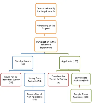
A total of 223 women participated in the behavioral experiments. This consisted of 153 applicants and 69 non-applicants. All participants in the behavioral experiments were randomly chosen.3 The experiments were conducted in the Pratham office located in South Shahdara, a prominent and convenient place for all the participants.
All women who applied to the program (applicants) and the non-applicants who participated in the experiments were followed-up at their homes and requested to participate in a household survey, which collected detailed information on household
demographic characteristics, schooling outcomes, assets, employment, labor market outcomes (full time and part time employment in the past 30 days), quality of life and involvement in decision making within the household.4 We were unable to collect survey data on 5% of the applicants and 15% of the non-applicants who participated in the behavioral experiments: 7 of the 153 applicants and 11 of the 69 non-applicants could either not be traced or did not want to participate in the survey. Hence we have complete data for 204 women (146 applicants and 58 non-applicants). Figure 1 presents the summary of the program design and the sample sizes for the different groups. We did not find any differences in the intrinsic characteristics between subjects who participated in the experiments and completed the survey and subjects who only participated in the experiments but did not complete the survey (see Table A1 in Appendix 1).5
3
We first decided on the maximum number of participants we wanted for the 12 sessions that we planned to conduct in July 2010. This was determined by time and funding constraints. We already had the addresses of the applicants. We used this list to randomly invite the applicants. We stopped inviting once the number of invitations reached 200. For the non-applicants, we stratified them by the local cluster numbers and within each cluster we randomly invited women who satisfied the eligibility criterion. We stopped inviting once the number of invitations reached 100. We use the census data (collected prior to advertising the program) to compare average grades of schooling and age of all non-applicants with that of non-applicants who participated in the behavioral experiment. We find that the two groups have similar average grades of schooling completed and age (these are the only two variables on which information was collected in our census). This suggests that our non-applicant sample is representative of the non-applicant population..
4
Due to the length of the household survey, it was not possible to administer the survey during the experiment.
5
2.2 Experimental Design
We conducted 12 sessions and each session lasted approximately 2 hours. Each subject participated in only one session. The average payment received from participation was Rs 203 (including a show-up fee of Rs 150).6 The experiments that we conducted fall under the category of artefactual field experiments, using the categorization developed by Harrison and List (2004).
Each subject participated in two behavioral games. The first game was designed to evaluate subjects’ attitudes towards risk (investment game). In this game, participants were endowed with Rs 50 and had the option to allocate any portion of their endowment to a risky asset that had a 50% chance of quadrupling the amount invested. The invested amount
could also be lost with a 50% probability. The subjects retained any amount that they chose not to invest.
The second game was designed to investigate the intrinsic competitiveness of subjects (competition game). The subjects were required to participate in a real-effort task, which determined their payoffs in the experiment. The real-effort task consisted of filling up 1.5 fl oz. zip lock bags with kidney beans (locally known as Rajma) in one minute. Prior to the task each subject had to choose one of two possible methods of compensation. They could choose a piece-rate compensation method, which depended solely on their own performance and they would receive Rs 4 for each correctly filled bag. Alternatively, they could choose a competition-rate compensation method where their earnings would depend on how they performed relative to a randomly chosen subject in the same session. A subject received Rs 16 per bag if she filled more bags than her matched opponent (see section 2.2.1
household survey data is missing and 0 otherwise. The explanatory variables include the set of intrinsic traits included in specification 3 in Table 3 (see below) and the interaction of these variables with applicant status. The results are presented in Table A2 in Appendix 1. None of the variables included in the set of explanatory variables (interacted or not) are statistically significant and the interaction terms are also not jointly statistically significant. We are therefore assured that non-response is not systematically related to intrinsic differences between applicants and non-applicants.
6
for a discussion of the matching process). If she filled fewer bags than her opponent, she received nothing. When choosing their compensation method, the subjects also had to guess their performance in the game, by answering questions on the number of bags they expected to be able to fill, and their expected relative rank based on their performance in the task.
In each session, only one of the games was chosen for payment purposes. The basic structure of each game is similar to the games used in previous studies (for example, Gneezy, Leonard and List, 2009). We chose the payoffs such that the returns from choosing the riskier alternative were comparable in the two games. In both the games, choosing the riskier outcome gave four times higher payoffs compared to the riskless option. Our choice
of the real-effort task was specific to our field conditions. While we did not want a task that might be more familiar to a particular sub-section of our subjects (that could bias their expectations about their performance in the game), we had to choose a task that was feasible for our subject population. This ruled out many of the familiar experimental tasks like computing sums, or word tasks since our participants (and indeed the population they are drawn from) are weak in these skills. Kidney beans comprise a staple diet in the region; women are used to handling the beans regularly (they take them out in bowls, clean them etc.) in the process of cooking and all our participants are likely to be equally familiar with this particular task.
2.2.1 Procedure
Subjects were randomly allocated IDs at the beginning of the session and asked to take a seat in one of the two rooms (Room 1 henceforth for expositional purposes). No communication was allowed during the session and the participants were informed of this. The instructions were read out aloud in Hindi.7 We also used visual aids while reading out the instructions, in the form of display charts (see Figures A1 and A2 in Appendix 2). To enhance comprehension and minimize anchoring-bias (see Ariely, Loewenstein and Prelec, 2003) the instructions that were read out had other examples, in addition to the one
7
displayed in the charts. The instructions for the investment game were read out first and after that the subjects were ushered into an adjoining room one-by-one where they made their individual allocation decisions in front of one of the experimenters. Prior to making their choices, every subject was asked a few questions to ensure her comprehension of the game. Once a subject had specified her investment choice, the experimenter asked her to elaborate on the reason behind her choice.
After participants had made their decision for the investment game, they were re-seated in Room 1 where the instructions for the competition game were read out. Once again visual charts were used to explain the process (see Appendix 2). The participants were also shown what constituted a correctly filled bag. At the end of the demonstration,
they were again asked to go one by one to the adjoining room and answer a set of questions to ensure their understanding of the game, measure their level of confidence, discover their preferred form of compensation (piece-rate or competition rate), and find the reason behind their choice of compensation method. Once all participants had answered the questions, they were re-seated in Room 1, and given one minute to fill as many zip lock bags as possible with the kidney beans provided. The experimenter announced the closure of the task after a minute was over. Next, the number of correctly filled bags for each participant was recorded.
Finally, a coin was tossed in front of the participants which determined the game to be used for payment. Participants were paid privately in the adjoining room. If the investment game was chosen for payment purposes, a second coin toss determined whether
While the same (female) experimenter read the instructions out aloud in every session, the questions were administered by two or three experimenters, depending on availability.8 Several of our subjects, despite having completed 5 or more grades of schooling, had poor reading and writing skills.9 The experimenters were therefore required to be actively involved in administering the questions and noting down the responses. Such a protocol clearly reduced the social distance between the subject and the experimenter, and could conceivably create scrutiny effects. It is useful to point out here that our main interest lies in the differences in the responses of applicants and non-applicants, and as long as any one of the groups is not systematically more affected by the scrutiny effect, any potential bias arising from the scrutiny effect will be differenced out. The fact that the decisions
taken in the games were not hypothetical and influenced by non-trivial monetary amounts, reinforced the contention that subject choices are minimally affected by social distance, and hence the choices should be viewed as real investment decisions. We think that our method is particularly relevant for field experiments run in developing countries where participating subjects might not have sufficient reading and writing skills.
The games were always run in the same order (i.e., the investment game, followed by the competition game), no feedback was provided to the subjects in between the two games and subjects were paid on the basis of the outcomes in one of the two tasks, randomly determined after all participants had finished participating in both games. The only task that a subject received any feedback for was the one for which they were paid. While the particular design choice meant that we cannot explicitly test for order effects, we anticipate that these effects would be minimized by paying for one game, with no feedback between games. Paying for one game also helped reduce wealth effects.
3. Results
3.1 Descriptive Statistics
8
An analysis of responses indicates that there are no differences depending on the gender of the experimenter administering the questions.
9
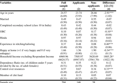
We start our analysis by discussing the demographic differences between the applicants and non-applicants gathered through our survey. Table 1 presents average individual and household characteristics for the sample of applicants and non-applicants. We also report t-tests for the mean differences in these characteristics. We find that program applicants are younger, are less likely to belong to the other backward class (OBC),10 have some prior experience of tailoring and stitching, come from relatively higher income households and are less likely to be happy at home. Of the 132 applicants who responded to this question, 52% reported that the main reason for applying to the program is to “increase future employment prospects”, followed by “like stitching” (24%) and “will help with
housework” (24%). We also find that 47% of the applicants (22% of the non-applicants)
are wives of the head of the household, 70% of the applicants (23% of the non-applicants) are daughters of the head of the household and finally 19% of the applicants (10% of the non-applicants) are daughters-in-law of the head of the household.
To measure respondents’ level of economic freedom as well as control over household resources, we asked in the survey whether the subject was able to choose/decide how to spend the money she has earned. We construct a variable “control over resources” that takes the value 1 if the respondent says yes and zero otherwise. We find that women with greater control over resources are significantly more likely to apply to the program. We also include an indicator for participation in a chit fund as an alternative measure of control over resources and using this measure, we find that while women with membership in a chit fund are more likely to apply to the program, the coefficient estimate is not statistically significant.11
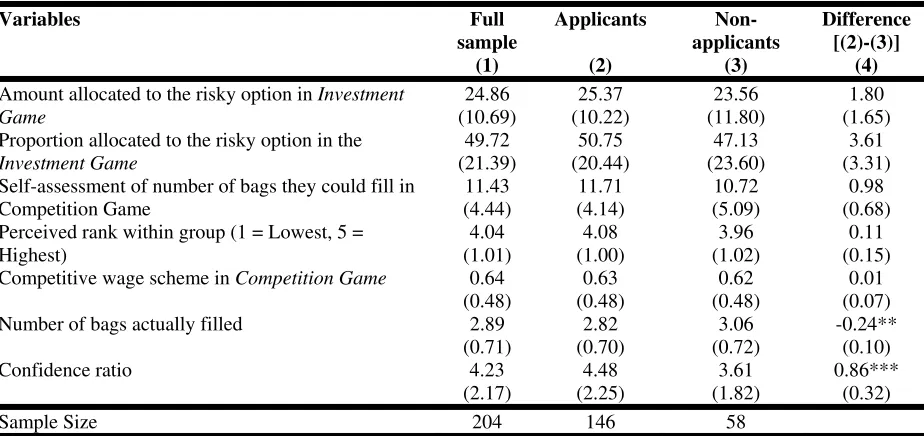
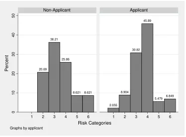
Table 2 reveals some interesting differences in intrinsic characteristics between the program applicants and non-applicants. Figure 2 presents the proportion of women
choosing to allocate Rs x to the risky investment in the investment game, where x ∈ {0, 1 – 10, 11 – 20, 21 – 30, 31 – 40, 41 – 50}. Approximately 58% of the applicants allocate more
10
The Central Government of India classifies some of its citizens based on their social and economic condition as Scheduled Caste, Scheduled Tribe and Other Backward Class (OBC).
11
than Rs 20 to the risky investment, compared to 43% of the non-applicants. If we use the amount invested in the risky asset as a measure of aversion to risk, then applicants appear to be less risk averse than non-applicants. The cumulative density function of the amount invested in the risky asset by applicants lies generally to the right of that of the non-applicants though clearly there is no stochastic dominance (Figure 3). Alternatively, the amount invested in the game can also be interpreted as a subject’s attitude towards loss aversion. Our results suggest that applicants are less loss-averse than the non-applicants.
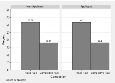
In the competition game though, 36.3% of the applicants and 36.2% of the non-applicants choose to be paid according to the competition rate, suggesting no difference in the attitude towards competition between the two groups (Figure 4). To further investigate
behavior in this game, we construct two measures of confidence: an absolute measure of confidence which is the subject’s estimate about the number of bags she would be able to fill in one minute, and a relative measure of confidence, which is the subject’s estimate about her relative standing (rank) vis-à-vis other participants in the session. Applicants in our sample appear to be more confident than the non-applicants using our measures of confidence (Table 2 and Figures 5 and 6). For example, Figure 5 shows that 52% of the non-applicants expected to fill more than 10 bags whereas more than 64% of the applicants thought they would do the same. These differences are however not statistically significant. The actual performance of non-applicants in the game (measured by the number of bags filled) was slightly better on an average (Table 2 and Figure 7). As figure 7 shows 81% of the non-applicants filled more than 2 bags as compared to 70% of applicants. This difference is not statistically significant.
by applicant status. While this function for the applicants lies to the right of that of non-applicants, the null hypothesis of no stochastic dominance cannot be rejected (p-value = 0.387).
Several other points are worth noting. First, the results presented in Table 2 suggest that the non-applicants are more likely to be unsure of their ability compared to the applicants. This is despite the fact that in the actual task they perform better (though the difference is not statistically significant). Second, in addition to eliciting competitive behavior, “competitiveness” can perhaps capture underlying preferences for a strategic risk. Choosing the competition rate as opposed to the piece-rate payment scheme can potentially be a risky alternative since payoffs in this case depend on the relative performance and not
absolute performance. We can therefore elicit two types of risk through our behavioral games. In the investment game the subject faces exogenous risk that is beyond her control, while in the competition game she faces risk that depends on her own performance, relative to that of other subjects. We do not find any systematic relationship between the risk category (as defined in Figure 2) and choice of the competition payment scheme in the competition game. Third, the choice of the payment scheme has a significant effect on
performance in the real-effort task. The average number of bags filled in one minute by women choosing the piece-rate compensation method is 2.8, compared to 3.05 for women who choose the competition-rate compensation method and this difference is statistically significant (p-value = 0.014).12 Finally, we find that women who choose the competition-rate compensation method are significantly more likely to place themselves at a higher rank within the group (correlation coefficient is 0.18 with a p-value = 0.007). This is not surprising, since in the competition-rate compensation method, they will earn a positive amount only if they fill more bags than their competitor and it seems logical to expect that a woman is likely to choose this method of compensation only if she believes herself to be better than others in the group. The choice of the compensation method is however not affected by their expectation of the number of bags they are likely to fill in the allotted one minute.
12
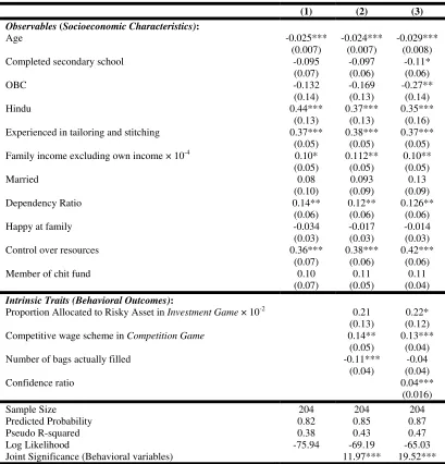
3.2 Regression results
We next estimate a multivariate regression model to capture the causal effects of the behavioral variables on the decision to apply to the program, controlling for the observable demographic characteristics. A probit model is estimated to characterize the determinants of program participation. The marginal effects and robust standard errors are reported in Table 3. Results corresponding to three different specifications are presented. In specification 1, we include only socio-economic characteristics obtained from the survey. In specification 2 we include the proportion of endowment allocated to the risky asset in the investment game and choice of the competitive wage scheme in the competition game as
additional controls. Finally in specification 3 we also control for confidence (measured by the confidence ratio). Specifications 2 and 3, in addition control for the actual performance in the real effort task (number of bags filled in the allotted one minute).
Including the intrinsic traits substantially improves the fit of the model as compared to specification 1, which only includes the observable variables. The predicted probability, the pseudo R-squared and the log likelihood are all higher in specifications 2 and 3. The behavioral variables are always jointly statistically significant in explaining applicant status. Our final preferred specification is reported in column 3 in Table 3, which includes the full set of observable and intrinsic traits.
Applicants and non-applicants differ along many observable characteristics. We find that age, religion and caste have an important role in explaining applicant status. Younger women are more likely to apply to the program: an additional year in age is associated with a 3 percentage point reduction in the probability of applying to the program. Hindu women are 35 percentage points more likely to apply to the program. Women belonging to the Other Backward Class (OBC) are 27 percentage points less likely to apply to the program. Married women are also more likely to apply to the program though this variable is not statistically significant.
outside options. The process of reforms in India over the last two decades have opened up significant opportunities for individuals with the right kinds of skills and educated women have benefitted the most from this (Munshi and Rosenzweig, 2006). Our results support this argument. Women with some prior experience in tailoring and stitching are 37 percentage points more likely to apply to the program.
Although the training program was administered free of cost, participation in the program needed significant time commitment, which can appear to the subjects as a high opportunity cost. To investigate further whether that is indeed the case, we include the variable dependency ratio, defined as the ratio of the number of children under 5 in a household and the number of adult females in the household. Conceivably, the dependency
ratio can influence behavior in two different ways. First, since women are typically the primary care-givers for children, a woman belonging to a household which has relatively more children compared to the available adult women faces a substantially higher time-cost of participating in the training program. In this case an increase in the dependency ratio will urge a participant to substitute away from the training program, and hence reduce the probability of applying to the program. On the other hand, it is often the case that in our subject-demographics, it is the woman’s responsibility to find the resources required to send children to school or take them to a doctor/hospital when they are sick. In this socio-economic set up it is not surprising then to find that most applicants report that the primary reason for applying to the program is to increase future income. Here, an increase in dependency ratio would put more pressure on the adult woman to seek out additional ways to support household income. We would then expect a positive relation between the increase in the dependency ratio and the probability of applying to the program due to the underlying income-earning motive. Which of the two effects is stronger is an empirical question. In our sample, we find that the income effect dominates the substitution effect.
control over resources (i.e. are able to choose how to spend money) are 42 percentage points more likely to apply to participate in the program. Being a member of a chit fund has a positive but not a statistically significant effect on the probability of applying to the program. We also notice that women who are happier at home are less likely to apply to the program, though this variable is not statistically significant.
Turning to the effects of the intrinsic traits, we find that women who are less risk averse (or are loss averse), more competitive and more confident of their ability are more likely to apply to the vocational training program. A one-percent increase in the proportion of the endowment allocated to the risky asset in the investment game is associated with a 0.22 percentage point increase in the probability of applying to the program. Women who
choose the competitive wage scheme in the competition game are 13 percentage points more likely to apply to the program. A unit increase in the confidence ratio is associated with a 4 percentage point increase in the probability of applying to the program.
We control for performance in the task to capture participant’s display of effort in the game. Interestingly it is the non-applicants who perform better in this specific real effort task with an additional bag filled in the real effort task, being associated with a 11 percentage points decrease in the probability of applying to the program.13
While most of the coefficient estimates are similar across the different specifications, failure to include the intrinsic traits in the regressions is associated with an omitted variable bias. For example, in specification 1 women belonging to OBC are 13 percentage points less likely to apply for the program and this effect is not statistically significant. This effect increases to 27 percentage points in specification 3 (a doubling of the effect) and is significant. Similarly a subject who has completed secondary school is 9.5 percentage point less likely to apply for the program (not statistically significant) in specification 1 and 11 percentage points more likely to apply in specification 3 (statistically significant).
13
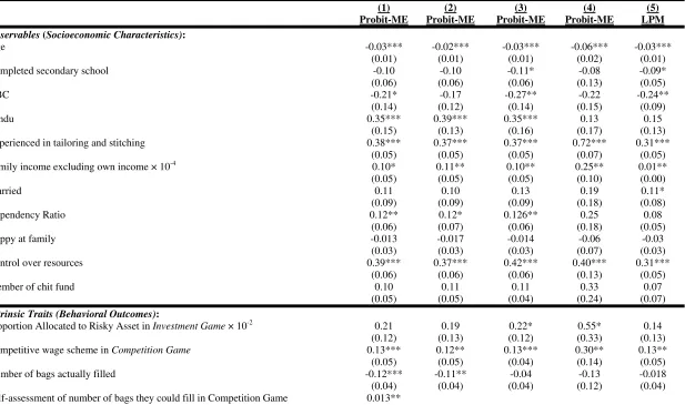
3.3. Robustness
We estimate several alternative specifications to ensure that the findings presented in Table 3 are robust. We discuss four robustness tests in this section. First, in specifications 1 and 2 in Table 4 we include alternative measures of confidence: self-assessment of the number of bags they could fill in the real effort task (specification 1) and perceived rank within the group (specification 2). In these two specifications we do not include confidence ratio as an additional explanatory variable. A unit increase in the number of bags the woman expects to be able to fill is associated with a 1.3 percentage points increase in the probability of applying for the program; a unit increase in the perceived rank within the group is associated with a 2.4 percentage point increase in the probability of applying for the
program (though in this case the effect is not statistically significant). The rest of the results remain qualitatively similar.
Second, in specification 3 we include time preference as an additional control (the rest of the explanatory variables are as in specification 3 in Table 3). The rate at which an individual discounts future pay-offs can influence the decision to be an applicant to the program. Returns from a vocational training program (and indeed from all educational programs) require a gestation lag to bear fruit (see for example Ray (2003) and Mullainathan (2005) for a discussion on how present bias can shape schooling decisions). It is possible that women who have a higher discount rate (are more present biased) might tend to discount the future returns from the program more heavily and choose not to apply. We capture time preference using a question in our household survey: the respondent is asked to choose between a sure prize of Rs 100 today versus Rs 150 one month from today. The variable present bias takes the value of 1 if the respondent chooses Rs 100 today.14 The results from specification 3 in Table 4 show that while the coefficient of the present bias dummy is in the expected direction, it is not statistically significant and the inclusion of this
14
variable does not have any effect on the other explanatory variables (compare specification 3 in Tables 3 and 4).
Third, our sample composition has some imbalance: the estimating sample consists of 58 non-applicants and 146 applicants. To examine if our results are sensitive to this imbalance, we re-run our preferred specification on a new sample, which consists of the non-applicants and a randomly chosen subset of the applicants. The estimating sample here consists of 58 non-applicants and 47 applicants.15 These results are reported in specification 4 in Table 4. We find that our results are qualitatively very similar though the magnitude of the coefficient estimates and the standard errors are higher.16
Fourth, women in the sample reside in a number of different clusters (within the
South Shahdara area of New Delhi). The presence of common cluster level unobservables could lead to incorrect inference. The most common solution for this would be to compute the cluster robust standard errors. The difficulty in our case is that the number of clusters from which our sample is drawn is small (only 11 in our sample), and therefore simply clustering the standard errors would not address this issue (see Woolridge, 2003). An alternative would be to estimate a linear probability model with cluster fixed effects and robust standard errors. This allows us to account for common cluster level unobservables. The corresponding estimates are reported in specification 5 in Table 4. We find that the magnitude and sign of all the coefficient estimates are similar and not different from our preferred estimates reported in specification 3 in Table 3.
4. Discussion
This paper uses a novel design that combines household survey data with unique experimental data to examine the determinants of self-selection into vocational training programs. Our approach allows us to identify both observable and selected intrinsic
15
Recall this data was collected as a part of a randomized training program and the applicants were randomly allocated into a control and a treatment group. The treatment group received the free 6 month training while the control group did not. These 47 applicants form the randomly chosen control group.
16
characteristics that separate the applicants from the non-applicants in our training program. We find that younger Hindu women, with prior experience in stitching and tailoring, belonging to households with higher income and dependency ratio and having control over resources have a significantly higher probability of applying to the training program offered. The results from our behavioral experiment reveal that women who are less risk averse, more competitive and more confident are more likely to apply to the training program.
There are several implications of our results. First, identifying the specific sources of intrinsic traits can help researchers address the selection issue better by specifically controlling for these characteristics instead of including them in the black box called
References:
[1] Anderson, S. and J-M. Baland (2002): “The Economics of Roscas and Intrahousehold Resource Allocation”, Quarterly Journal of Economics, 117(3), 963 – 995.
[2] Andersen, S., S. Ertac, U. Gneezy, J. List and S. Maximiano (2010): Gender, Competitiveness and Socialization at a Young Age: Evidence from a Matrilineal and a Patriarchal Society, Mimeo University of Chicago.
[3] Ariely, D., G. Loewenstein and D. Prelec (2003): “Coherent Arbitrariness: Stable Demand Curves without Stable Preferences”, Quarterly Journal of Economics, 118(1), 73 – 105.
[4] Attanasio, P. O., A. D. Kugler and C. Meghir (2011): “Subsidizing Vocational Training for Disadvantaged Youth in Colombia: Evidence from a Randomized Trial”, American Economic Journal: Applied Economics, 3(2), 188-220.
[5] Belzil, C. and M. Leonardi (2009): Risk Aversion and Schooling Decisions, Ecole Polytechnique, Working Paper # 2009-028.
[6] Bénabou, R. and J. Tirole (2002): “Self Confidence and Personal Motivation”, Quarterly Journal of Economics, 117(3), 871 – 915.
[7] Bernardo, A. E., and Welch, I. (2001): “On the Evolution of Overconfidence and Entrepreneurs”, Journal of Economics and Management Strategy, 10(3), 301 – 330.
[8] Betcherman, G., K. Olivas and A. Dar (2004): Impacts of Active Labor Market Programs: New Evidence from Evaluations with Particular Attention to Developing and Transition Countries, World Bank Social Protection Discussion Paper # 0402.
[9] Biais, B., D. Hilton, K. Mazurier and S. Pouget (2005): “Judgemental Overconfidence, Self-Monitoring, and Trading Performance in an Experimental Financial Market”, Review of Economic Studies, 72(2), 287 – 312.
[10]Camerer, C. F., and D. Lovallo (1999): “Overconfidence and Excess Entry: An Experimental Approach”, American Economic Review, 89, 306 – 318.
[11]Card, D., P. Ibarraran, F. Regalia, D. Rosas and Y. Soares (2011): “The Labor Market Impacts of Youth Training in the Dominican Republic: Evidence from a Randomized Evaluation”, Journal of Labor Economics, forthcoming.
[12]Cardenas, J. C. and J. Carpenter (2008): “Behavioural Development Economics: Lessons from the Field Labs in the Developing World”, Journal of Development Studies, 44(3), 311 – 338.
[13]Castillo, M, R. Petrie and M. Torero (2010): “On the Preferences of Principals and Agents”, Economic Inquiry, 48(2), 266 – 273.
[14]Chen, S. (2003): Risk Attitude and College Attendance, Mimeo, SUNY Albany.
[15]Filippin, A. and M. Paccagnella (2009): Family Background, Self-Confidence and Economic Outcomes, Mimeo.
[16]Cooper, A. C., C. A. Woo and W. Dunkelberg (1988): “Entrepreneurs Perceived Chances for Success,” Journal of Business Venturing, 3, 97 – 108.
[17]Eriksson, T., S. Teyssier and M. C. Villeval (2009): “Self-Selection and the Efficiency of Tournaments”, Economic Inquiry, 47(3), 530 – 548.
[18]Fang, H. and G. Moscarini (2005): “Morale hazard”, Journal of Monetary Economics, 52(4), 749 – 777. [19]Gneezy, U., K. L. Leonard and J. List (2009): “Gender Differences in Competition: Evidence from a
Matrilineal and Patriarchal Society”, Econometrica, 77(5), 1637 – 1664.
[20]Grubb, W.N. (2006): Vocational Education and Training: Issues for a Thematic Review”, OECD. [21]Harrison, G. W, M. Lau and M. B. Williams (2002): “Estimating Individual Discount Rates in Denmark:
A Field Experiment”, American Economic Review, 92(5), 1606 – 1617.
[22]Harrison, G. W. and J. List (2004): “Field Experiments”, Journal of Economic Literature, b, 1009 – 1055.
[24]Heckman, J. J., R. J. Lalonde and J. A. Smith (1999): “The Economics and Econometrics of Active Labor Market Programs” in Handbook of Labor Economics, Volume III, O. Ashenfelter and D. Card (ed). Amsterdam, North-Holland.
[25]Koszegi, B., (2006): “EgoUtility, Overconfidence, and Task Choice,” Journal of the European Economic Association, 4(4), 673 – 707.
[26]Koellinger, P., M. Minniti and C. Schade (2007): “`I think I can, I think I can’: Overconfidence and Entrepreneurial Behavior”, Journal of Economic Psychology, 28, 502 – 527.
[27]Liu, E. M. (2008): Time to Change What to Sow: Risk Preferences and Technology Adoption Decisions of Cotton Farmers in China, Working Paper #1064, Princeton University, Department of Economics, Industrial Relations Section.
[28]Mullainathan, S. (2005): “Development Economics through the Lens of Psychology” in Lessons of experience: Annual World Bank Conference on Development Economics.
[29]Moore, D. A., and Healy, P. J. (2008): “The trouble with overconfidence”, Psychological Review,
115(2), 502 – 517.
[30]Munshi, K. and M. Rosenzweig (2006): “Traditional Institutions Meet the Modern World: Caste, Gender and Schooling Choice in a Globalizing Economy”, American Economic Review, 96(4), 1225 – 1252. [31]Niederle, M. and L. Vesterlund (2007): “Do Women Shy away from Competition? Do Men Compete too
Much?,” Quarterly Journal of Economics, 122(3), 1067 – 1101.
[32]Ray, D. (2003): Aspiration, Poverty and Economic Change. BREAD Policy Paper # 2.
Table 1: Summary Statistics on Socioeconomic Characteristics Variables Full sample (1) Applicants (2) Non-applicants (3) Difference [(2)-(3)] (4)
Age in years 24.57
(6.69) 23.74 (5.93) 26.66 (7.99) -2.91*** (1.02)
Married 0.49
(0.50) 0.47 (0.50) 0.55 (0.50) -0.07 (0.07)
Completed secondary school (class 10 in India) 0.43
(0.49) 0.42 (0.49) 0.44 (0.50) -0.02 (0.07) OBC 0.10 (0.30) 0.07 (0.26) 0.17 (0.38) -0.10** (0.04) Hindu 0.97 (0.16) 0.97 (0.14) 0.94 (0.22) 0.03 (0.02)
Experience in stitching/tailoring 0.37
(0.48) 0.48 (0.50) 0.08 (0.28) 0.40*** (0.06) Happy at home (=1 if very happy and 0 if very
unhappy) 1.66 (0.91) 1.56 (0.80) 1.90 (1.11) -0.34*** (0.13)
Household Income excluding Respondent Income 6969.96
(6624.57) 7505.97 (6947.07) 5620.69 (5561.70) 1885.28* (1022.18) Dependency Ratio (no. of children under 5 years
divided by the no. of adult females)
0.31 (0.51) 0.35 (0.55) 0.22 (0.38) 0.12 (0.07)
Control over resources 0.57
(0.49) 0.67 (0.47) 0.34 (0.47) 0.33*** (0.07)
Member of chit fund 0.10
(0.31) 0.13 (0.33) 0.05 (0.22) 0.07 (0.04)
Sample size 204 146 58
In columns 1, 2 and 3, standard deviation reported in parenthesis and in column 4, standard error in parenthesis.
Table 2: Summary Statistics on Behavioral Outcomes Variables Full sample (1) Applicants (2) Non-applicants (3) Difference [(2)-(3)] (4)
Amount allocated to the risky option in Investment Game 24.86 (10.69) 25.37 (10.22) 23.56 (11.80) 1.80 (1.65) Proportion allocated to the risky option in the
Investment Game
49.72 50.75 47.13 3.61
(21.39) (20.44) (23.60) (3.31)
Self-assessment of number of bags they could fill in Competition Game 11.43 (4.44) 11.71 (4.14) 10.72 (5.09) 0.98 (0.68) Perceived rank within group (1 = Lowest, 5 =
Highest) 4.04 (1.01) 4.08 (1.00) 3.96 (1.02) 0.11 (0.15) Competitive wage scheme in Competition Game 0.64
(0.48) 0.63 (0.48) 0.62 (0.48) 0.01 (0.07)
Number of bags actually filled 2.89
(0.71) 2.82 (0.70) 3.06 (0.72) -0.24** (0.10)
Confidence ratio 4.23
(2.17) 4.48 (2.25) 3.61 (1.82) 0.86*** (0.32)
Sample Size 204 146 58
In columns 1, 2, and 3 standard deviations are reported in parenthesis and in column 4, standard error in parenthesis.
Table 3: Determinants of Applicant Status: Marginal Effects from Probit Regression
(1) (2) (3)
Observables (Socioeconomic Characteristics):
Age -0.025*** -0.024*** -0.029***
(0.007) (0.007) (0.008)
Completed secondary school -0.095 -0.097 -0.11*
(0.07) (0.06) (0.06)
OBC -0.132 -0.169 -0.27**
(0.14) (0.13) (0.14)
Hindu 0.44*** 0.37*** 0.35***
(0.13) (0.13) (0.16)
Experienced in tailoring and stitching 0.37*** 0.38*** 0.37***
(0.05) (0.05) (0.05)
Family income excluding own income × 10-4 0.10* 0.112** 0.10**
(0.05) (0.05) (0.05)
Married 0.08 0.093 0.13
(0.10) (0.09) (0.09)
Dependency Ratio 0.14** 0.12** 0.126**
(0.06) (0.06) (0.06)
Happy at family -0.034 -0.017 -0.014
(0.03) (0.03) (0.03)
Control over resources 0.36*** 0.38*** 0.42***
(0.07) (0.06) (0.06)
Member of chit fund 0.10 0.11 0.11
(0.07) (0.05) (0.04)
Intrinsic Traits (Behavioral Outcomes):
Proportion Allocated to Risky Asset in Investment Game× 10-2 0.21 0.22*
(0.13) (0.12)
Competitive wage scheme in Competition Game 0.14** 0.13***
(0.05) (0.04)
Number of bags actually filled -0.11*** -0.04
(0.04) (0.04)
Confidence ratio 0.04***
(0.016)
Sample Size 204 204 204
Predicted Probability 0.82 0.85 0.87
Pseudo R-squared 0.38 0.43 0.47
Log Likelihood -75.94 -69.19 -65.03
Joint Significance (Behavioral variables) 11.97*** 19.52***
Robust standard errors in parentheses
Table 4: Robustness
(1) (2) (3) (4) (5) Probit-ME Probit-ME Probit-ME Probit-ME LPM
Observables (Socioeconomic Characteristics):
Age -0.03*** -0.02*** -0.03*** -0.06*** -0.03***
(0.01) (0.01) (0.01) (0.02) (0.01)
Completed secondary school -0.10 -0.10 -0.11* -0.08 -0.09*
(0.06) (0.06) (0.06) (0.13) (0.05)
OBC -0.21* -0.17 -0.27** -0.22 -0.24**
(0.14) (0.12) (0.14) (0.15) (0.09)
Hindu 0.35*** 0.39*** 0.35*** 0.13 0.15
(0.15) (0.13) (0.16) (0.17) (0.13)
Experienced in tailoring and stitching 0.38*** 0.37*** 0.37*** 0.72*** 0.31***
(0.05) (0.05) (0.05) (0.07) (0.05)
Family income excluding own income × 10-4 0.10* 0.11** 0.10** 0.25** 0.01**
(0.05) (0.05) (0.05) (0.10) (0.00)
Married 0.11 0.10 0.13 0.19 0.11*
(0.09) (0.09) (0.09) (0.18) (0.08)
Dependency Ratio 0.12** 0.12* 0.126** 0.25 0.08
(0.06) (0.07) (0.06) (0.18) (0.05)
Happy at family -0.013 -0.017 -0.014 -0.06 -0.03
(0.03) (0.03) (0.03) (0.07) (0.03)
Control over resources 0.39*** 0.37*** 0.42*** 0.40*** 0.31***
(0.06) (0.06) (0.06) (0.13) (0.05)
Member of chit fund 0.10 0.11 0.11 0.33 0.07
(0.05) (0.05) (0.04) (0.24) (0.07)
Intrinsic Traits (Behavioral Outcomes):
Proportion Allocated to Risky Asset in Investment Game × 10-2 0.21 0.19 0.22* 0.55* 0.14
(0.12) (0.13) (0.12) (0.33) (0.13)
Competitive wage scheme in Competition Game 0.13*** 0.12** 0.13*** 0.30** 0.13**
(0.05) (0.05) (0.04) (0.14) (0.05)
Number of bags actually filled -0.12*** -0.11** -0.04 -0.13 -0.018
(0.04) (0.04) (0.04) (0.12) (0.04)
(0.006)
Perceived rank within group (1 = Lowest, 5 = Highest) 0.024
(0.02)
Present Bias -0.03
(0.05)
Confidence ratio 0.04*** 0.08** 0.04***
(0.016) (0.04) (0.01)
Sample Size 204 204 204 105 204
Predicted Probability 0.86 0.85 0.87 0.43
Pseudo R-squared 0.44 0.43 0.47 0.46
R-squared 0.45
Log Likelihood -67.06 -68.85 -64.29 -39.28
Joint Significance (Behavioral variables) 17.26*** 12.36*** 20.38*** 11.93** 3.70***
Robust standard errors in parentheses.
*** p<0.01, ** p<0.05, * p<0.1.
Specifications 1 – 4 present the marginal effects from probit regressions.
Figure 2: Amount Allocated to the Risky Asset, by Applicant Status
Note: Risk categories: 1= Rs 0; 2 = Rs 1 – 10; 3 = Rs 11 – 20; 4 = Rs 21 – 30; 5 = Rs 31 – 40; 6 = Rs 41 – 50. The risk categories capture the amount invested in the lottery, that is, risky asset.
20.69 36.21
25.86
8.621 8.621
2.055 8.904
30.82 45.89
5.479 6.849
0
10
20
30
40
50
1 2 3 4 5 6 1 2 3 4 5 6
Non-Applicant Applicant
Pe
rcen
t
Figure 3: CDF Percentage Invested in Risky Asset, by Applicant Status
0
.2
.4
.6
.8
1
CD
F
0 10 20 30 40 50 60 70 80 90 100
Percentage Invested in Risky Asset
Figure 4: Competitive Wage Scheme in Competition Game, by Applicant Status
63.79
36.21
63.7
36.3
0
10
20
30
40
50
60
70
80
Piece Rate Competitive Rate Piece Rate Competitive Rate
Non-Applicant Applicant
Pe
rcen
t
Figure 5: Self Assessment of Number of Bags they expect to fill, by Applicant Status
17.24 31.03
37.93
13.79
6.849 28.77
51.37
13.01
0
20
40
60
1 - 5 6 - 10 11 - 15 16 - 20 1 - 5 6 - 10 11 - 15 16 - 20
Non-Applicant Applicant
Pe
rcen
t
Figure 6: Perceived Rank Within Group by Applicant Status
1.724 6.897
22.41
31.03 37.93
2.055 3.425
23.97 25.34 45.21
0
50
1 2 3 4 5 1 2 3 4 5
Non-Applicant Applicant
Pe
rce
n
t
Figure 7: Number of Bags Actually Filled, by Applicant Status
18.97 58.62
18.97
3.448
2.055 28.08
56.16
13.01
.6849
0 20 40 60
0 1 2 3 4 5 0 1 2 3 4 5
Non-Applicant Applicant
Percent
Number of actual bags filled
Figure 8: CDF of Confidence, by Applicant Status
0
.2
.4
.6
.8
1
CD
F
0 1 2 3 4 5 6 7 8 9 10 11 12 13
Measure of Overconfidence
Appendix 1:
Table A1: Summary Statistics of Behavioral Outcomes by Missing and Non-missing Survey Data Sample without missing survey data (1) Sample with missing survey data (2) Difference [1-2] (3)
Amount allocated to the risky option in Investment Game 24.86 (10.69)
24.44 (10.55)
0.41 (2.62) Proportion allocated to the risky option in the Investment Game 49.72
(21.39)
48.88 (21.11)
0.83 (5.25) Self-assessment of number of bags they could fill in
Competition Game 11.43 (4.44) 11.00 (3.85) 0.43 (1.08) Perceived rank within group (1 = Lowest, 5 = Highest) 4.04
(1.01)
3.88 (1.18)
0.16 (0.25) Piece-rate wage scheme in Competition Game 0.65
(0.48)
0.72 (0.46)
-0.08 (0.11)
Number of bags actually filled 2.89
(0.71) 3.00 (1.02) -0.10 (0.18) Confidence 4.23 (2.17) 3.85 (1.33) 0.37 (0.52)
Sample Size 204 18
Table A2: Non-Response in Surveys: Marginal Effects from Probit Regressions
Covariates Non-response
Proportion allocated to the risky option in the Investment Game (× 10-2) 0.0097 (0.096)
Competitive wage scheme in Competition Game -0.028
(0.048)
Number of bags actually filled -0.00008
(0.036)
Confidence 0.0088
(0.010)
Applicant status (=1 if applicant) -0.074
(0.26) Proportion allocated to the risky option in the Investment Game × Applicant
status
0.0004 (0.0013) Competitive wage scheme in Competition Game × Applicant status -0.0014 (0.06)
Number of bags actually filled × Applicant status -0.010
(0.05)
Confidence × Applicant status -0.019
(0.016)
Observations 222
Robust standard errors in parentheses
*** p<0.01, ** p<0.05, * p<0.1
Appendix 2: English Version of the Subject Instructions
General Instructions
Player ID #: __________________________
Thank you for your participation. You will be paid Rs. 150 for your participation. There are 2 tasks that we will ask you to participate in. Performing each task can win you more money in cash, in addition to the guaranteed Rs. 150.
Although, each of you will complete both the tasks, only one of them will be chosen for payments. I will toss a coin at the end of the two tasks in front of everyone to determine the task you will be paid for. Note that everyone will be paid according to their performances in the task determined by the coin toss.
We are about to begin the first task. Please listen carefully. It is important that you understand the rules of the task properly. If you do not understand, you will not be able to participate effectively. We will explain the task and go through some examples together. There is to be no talking or discussion of the task amongst you. There will be opportunities to ask questions to be sure that you understand how to perform each task. At any time whilst you are waiting during this experiment, please remain seated, and do not do anything unless instructed by the experimenter. Also do not look at others responses at any time during this experiment.
Finally, each page has an ID# on it. Do not show this ID# to any other participant or allow it to be visible to anyone during or after this experiment.
Instructions for the Investment Game
Player ID #: __________________________
We are about to begin the first task. Please listen carefully to the instructions.
In this task, you are provided Rs.50. You have the opportunity to invest a portion of this amount (between Rs.0 and Rs.50). No money will be given at this point. All actual payments will be made at the end of the experiment if this task is chosen as the one that you will be paid for.
The investment:
There is an equal chance that the investment will fail or succeed. If the investment fails, you lose the amount you invested. If the investment succeeds, you receive 4 times the amount invested.
How do we determine the outcome of the investment:
After you have chosen how much you wish to invest, you will toss a coin to determine whether your investment has failed or succeeded, if this task is chosen for payment. If the coin comes up heads, you win four times the amount you chose to invest. If it comes up tails, you lose the amount invested. You will toss the coin at the end of the experiment, when you come to collect your payment.
Here are some examples:
1. You choose to invest nothing. You will get Rs.50 for sure if this task is chosen for payment.
2. You choose to invest all of the Rs.50. Then if the coin comes up heads, you get Rs.200. If the coin comes up tails, you get Rs.0.
Do you have any questions? If you are ready, we will proceed.
We will call each of you one at a time in the adjoining areas where you will be asked a few questions and participate in the described task.
Decision Sheet for the Investment Game
Please complete the example below:
1. If you choose to invest Rs 15 and the coin toss comes up heads, what will you receive?
Rs______ x ______ = Rs______
Actual Decision:
2. Amount that I wish to invest: _______________________
3. Reason for this decision:
Instructions for the Competition Game
Player ID #: __________________________
We are about to begin the next task. Please listen carefully to the instructions. All the money that you earn from this task is yours to keep and will be given to you at the end of this experiment if this task is chosen as the one that you will be paid for.
For this Task, you will be asked to fill bags with Rajma beans and seal it so its contents remain securely inside. We will give a demonstration before you start the task.
You will be given 1 minute to fill up as many bags as you can. Only bags filled and properly sealed will be counted towards your payments.
You can choose one of two payment options for this task.
Option 1:
If you choose this option, you get Re. 4 for each bag that you fill properly in 1 minute.
Option 2:
If you choose this option, you will be randomly paired with another person and your payment depends on your performance relative to that of the person that you are paired with. If you fill up more bags properly than the person you are paired with, you will receive Rs.16 per bag that you filled. If you both fill the same number of bags you will receive Rs. 16 per bag. If you fill up less number of bags than the person you are paired with, you will receive Rs. 0.
Note that what you will earn does not depend on the decision of the person that you are paired with; it only depends on your own choice of payment, your performance and their performance.
Here are some examples of what could happen:
1) You choose option 1. You fill 10 bags properly. You will receive 10xRe. 4 = Rs. 40.
2) You choose option 2. You fill 3 bags properly. The person that you are paired with fills 2 bags properly. You will receive 3xRs.16 = Rs. 48.
3) You choose option 2. You fill 3 bags properly. The person that you are paired with fills 4 bags properly. You will receive 3 x 0 = Rs. 0.
Note that these are examples only. The actual decision is up to you.
Next, we will call each of you one at a time in the adjoining area where you will be asked a few questions and choose your preferred option in the above described task. Once you have answered the questions and indicated your preferred option, you will come back to your sitting area. Please make sure that you do not converse with anyone at this time. If we find you conversing you will be disqualified from further participation and escorted out by one of the experimenters.
Once everyone is back to the seating area we will announce the start of the task and you can start filling up the bags. We will make an announcement when there are 30 seconds remaining. When time is up, we will say, “Stop the task now”. You should immediately
stop filling the bags. Please make sure that your hands are in your lap now and not touching any of the bags that you filled up. If you do not do this within 2 seconds, you will receive Rs. 0 for the entire experiment.
We will come around and inspect the bags and record the number of bags filled each of you managed to fill up.
Once all counting is done we will flip a coin to decide which of the two tasks will be chosen for payments.
After the coin toss, each of you will be again called one at a time to the adjoining area for the final payment procedures.
Decision Sheet for the Competition Game
Player ID #: ____________________
Questions for Task # 2
Please answer the following questions:
1. Suppose you choose Option 1. You complete 11 bags correctly at the end of 1 minute. How much money do you receive?
_______ x Rs________ = ________________
2. Suppose you choose Option 2. You complete 7 bags correctly. The person you are paired with completes 6 bags correctly. How much money do you receive?
_______ x Rs________ = ________________
3. How many bags do you think you can fill properly in 1 minute? _____________________
4. If we were to rank everyone’s performance, in the group of people in this room, from best to worst, where do you think you would fall compared to the average person? Please place a tick next to the rank that you think applies to you.
__ 1-4 (very above average)
__ 5-8 (above average)
__ 9-12 (average)
__13-16 (below average)
__ 17-20 (very below average)
5. We now ask you to choose how you want to be paid: according to option 1 or option 2? _____________________
6. What was your decision based on?
Performance Sheet for Task 2
No. of bags filled: _________________________________
Player ID #: ____________________
For experimenter use only
Instructions for Final Payment Determination
We will now determine what task to pay you for. We will flip a coin; you will all be paid for task 1 if Heads come and task 2 if Tails come up.
If Head comes up, then Task 1 is chosen: Each one of you will flip a coin to determine whether your investment succeeded or not. If the coin comes up heads, you win four times the amount you chose to invest. If it comes up tails, you lose the amount invested.
If Tail comes up then Task 2 is chosen: We will pay you according to the choice you had indicated earlier.
If you had chosen option 1, we will pay you according to your performance.
If you had chosen option 2, we will ask you to pick one chit amongst several chits of paper on the front desk. Each chit contains an id number of one of the participants. Your performance will be matched with the performance of the participant whose ID number you picked. You will be paid according to your relative performance as described earlier.
Visual Charts