© 2015, IRJET ISO 9001:2008 Certified Journal Page
448
PARAMETER IDENTIFICATION OF PMSM USING LSA METHOD
A. Swathi
1, P. Ramana
21
PG student, Department of EEE, GMR I T Rajam, Srikakulam, AP, India
2Associate Professor, Department of EEE, GMR I T Rajam, Srikakulam, AP, India
---***---Abstract -
In the last 20 years Permanent MagnetSynchronous Machine (PMSM) are becoming more indispensable in many industrial applications. The PMSM is superior to both induction motor drives and DC motor drives because of the inherent advantages of these motors include high efficiency, high power factor, high power density, easy maintenance, fast dynamic response, and the minimum magnet cost because of low magnet weight requirement. Parameter identification is necessity to get good performance of PMSM drive. Here least square approximation is used find the parameters of motor such as stator inductance and resistance, viscous coefficient and inertia constant without any sensors and encoders. Many advantages of sensor less control such as reduced hardware complexity, low cost, reduced size, cable elimination, increased noise immunity, increased reliability and decreased maintenance.
Key Words:
permanent magnet AC motor, parameter
estimation, least square approximation
1. INTRODUCTION
The permanent-magnet synchronous machine (PMSM) drive has emerged as a top competitor for a full range of motion control applications [1]-[3]. For example, the PMSM is widely used in machine tools, robotics, actuators, and is being considered in high-power applications such as vehicular propulsion and industrial drives. It is also becoming viable for commercial/residential applications. The PMSM is known for having high efficiency, low torque ripple, superior dynamic performance, and high power density. These drives often are the best choice for high-performance applications and are expected to see expanded use as manufacturing costs decrease. The purpose of this paper is to introduce the PMSM and the application of power electronics technology to its control.
The PMSM is sometimes referred to as a permanent-magnet AC (PMAC) machine or simply as a PM machine. In some instances it is referred to as a brushless DC (BDC) machine because by appropriate control it can be made to have input/output characteristics much like a separately excited brush-type DC machine [4]-[5]. It can also take on similarity with the DC machine when Hall Effect sensors are utilized for position sensing, whereby electronic, instead of brush, commutation take place. The
PMSM is a synchronous machine in the sense that it has a multiphase stator and the stator electrical frequency is directly proportional to the rotor speed in the steady state [6]. However, it differs from a traditional synchronous machine in that it has permanent magnets in place of the field winding and otherwise has no rotor conductors. The use of permanent magnets in the rotor facilitates efficiency, eliminates the need for slip rings, and eliminates the electrical rotor dynamics that complicate control (particularly vector control). The permanent magnets have the drawback of adding significant capital cost to the drive, although the long term cost can be less through improved efficiency. The PMSM also has the drawback of requiring rotor position feedback by either direct means or by a suitable estimation system. Since many other high performance drives utilize position feedback, this is not necessarily a disadvantage. Another disadvantageous aspect of the PMSM is cogging torque, which is the parasitic tendency of the rotor to align at discrete positions due to the interaction of the magnets and the stator teeth. Cogging torque is particularly Troublesome at low speed, but can be virtually eliminated either by appropriate design of the machine or by electronic mitigation. In contrast to the mentioned methods, a hybrid rotor design allows open-loop control from an inverter without rotor position feedback. This simple control method is suggested to replace conventional induction motors in applications like fans, pumps and ventilation systems where high dynamic performance is not a requirement.
2. NEED OF PARAMETER ESTIMATION
© 2015, IRJET ISO 9001:2008 Certified Journal Page
449
The Parameter Identification Method has followingadvantages
Time and money that is involved in testing process is saved as no mechanical coupling necessary.
Entire system information: it provides full information about characteristic curve and values of any motor.
3. PMSM MODEL
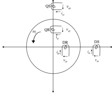
The design of the control system for a high performance drive requires a mathematical model of the motor. This is usually derived from the physical principles. Mathematical model of any machine can be developed by choosing reference frame, Park’s transformation and generalized model of the machine (i.e. Kron’s Primitive Machine), which can be utilized to control entire system in a simple manner [1-3]. The model of any machine can be implemented by set of its voltage equations, currents, fluxes, speed and torque. Mathematical model is usually derived from physical principles. The dynamics of a permanent magnet synchronous motor can be described by set of differential equations relating voltages, currents (fluxes), speed and torque. The equations represented in d-q axes variables in the rotor reference frame using park’s transformation are presented.
The voltage equations for the permanent magnet motor in rotor reference frame are
aqs qs qs aq qr r dsds r ad dr r
qs ri l pi l pi l i l i
v
(1) qr aq r qs qs r dr ad ds ds ds a
ds
r
i
l
pi
l
pi
l
i
l
i
v
(2) qs aq qr qr qr qr
qr
r
i
l
pi
l
pi
v
(3) ds ad dr dr dr dr
dr
r
i
l
pi
l
pi
v
(4) Where, Ψ = ladifr= air gap flux linkager t
e m
a
T
i
G
i
P
[
]
]
[
2 2 3 dr qs ad qr ds aq ds qs ds qs ds qs Pe
l
i
i
l
i
i
l
i
i
l
i
i
T
(5) The torque balance equation is,(6)
And the load torque for the no. of poles P=4 becomes;
) 2 1 ) 2 1 ] ) (
3 ad aq dsqs r r
l l l i i Jp
T
(7)To estimate currents, a model derived from the physical model of the machine is used. This model takes the following electrical properties into account:
Resistance of the phase windings,
Voltage induced by the rotating magnetic field of the rotor magnets
The inductivity of the phase windings
DS DR QR QS ds v dr v qs v r
vqr
ds i dr i qr i qs i
Fig -1: Basic two pole machine of PMS
The model does not treat the following things:
Eddy currents
Resistance change of the phase windings caused by thermal effects
Non-linear magnetic saturation and hysteresis effects of the iron parts
Magnetic working point changes caused by the temperature change of the rotor magnets.
These effects can also be taken into consideration in a more complex model, but even with a simple model good results can be achieved. The model describes the PMSM assuming: resistance value of every phase coils are equal, the rotor magnets generate sinusoidal voltage signals, and the inductivity of the coils can be described using (1). The most simple model is described in a coordinate system, where the two axes (d,q) are fixed to the magnetic axis of the rotor. Electrical model of the machine in this coordinate system can be seen. Where Id, Iq are the currents, Vd,Vq are the voltage inputs, Rs is the phase resistance, Ld and Lq are the direct and quadrature inductivities of the machine [7]. By neglect the inaccessible quantities such as damper winding and non liner terms (contains two states) the modeling equations becomes;
)
(
1
q qsq
v
Ri
L
di
(8))
(
1
d ds
d
v
Ri
L
di
(9)r r l e
d
j
T
T
2
2
(or) r r le
T
jd
T
)
(
2
(10)r r l e
d
j
T
T
2
2
(or) r r le
T
jd
T
)
(
2
(11)r l e r P T T Jp
P
2
[image:2.595.340.523.106.263.2]© 2015, IRJET ISO 9001:2008 Certified Journal Page
450
4. LEAST SQUARE APPROXIMATION METHOD
One of the most popular techniques for Parameter identification is the least square method (LSM) [8]-[9]. The various reasons for the popularity of method is firstly it works well with simple linear models secondly it make use of squares that make LSM tractable because according to the Pythagorean theorem if the error is independent of an estimated quantity, a squared error or the squared quantity can be added . Also the mathematical formulations and algorithms involved in LSM such as derivatives, Eigen decomposition, and singular value decomposition are easy and well known to use.
The LSM is basically used for finding the numerical values of parameters that best fit the curve data. It states that the most accurate value for the unknown quantities will be those for which the sum of the squares of the differences between the observed and the computed values is minimum and this difference between the estimated and calculated values is termed as residual .It uses the sum of squared of the difference b/w the obtained and predicted results.
Below equation shows the linear equation to be applied to entire system is that;
AX
Y
(12) But in case of nonlinear equations below equation to be used,bX
a
Y
(13)]
)
(
[
)
(
Y
iY
2Y
ia
bx
i 2E
(14)There are several types of LSM are to be presented. The simple form of Least square method [13] is known as Ordinary Least square method (OLS), And another version is called weighted least squares (WLS) and has better performance than OLS as it can modulate the final observation at the end of result .Some other variation in the least square method are alternating least squares (ALS) type and partial least squares (PLS) type [10].
4.1 RECURSIVE LEAST SQUARES
Recursive least squares is used for the parameters identification from recurring (in time) linear algebraic equations [11]. It is more robust and efficient than least square method .Since it does not make use of squares it is not sensitive to outranges as compared to least square method.
Consider a simple linear algebraic equation for a given set of time t
)
(
)
[image:3.595.323.547.427.529.2](
....
...
)
(
2
)
(
1 21
t
x
a
t
x
an
t
x
b
t
a
n
(15)Where aj(t) (j = 1, 2, ... , n) and b(t) = known data values xj (j = 1, 2, ... , n) = unknown parameters (to be calculated) .
Writing this equation in matrix-vector form, we get
0 0 0
X
b
A
(16) A0 represents aij = ai(tj), (i = 1, 2, ..., n; j = 1, 2, ..., m), x0 includes xj (j = 1, 2, ..., n), and b0Represents bi (i = 1, 2...m). The solution after applying least square method to Eq. (16) is
0 0 1 0 0
0
(
A
A
)
A
b
X
T T (17) Let after time tm+1 the equation changes to)
(
)
(
..
...
)
(
)
(
1 1 2 2 2 11
t
mx
a
t
mx
a
nt
mnx
n
b
t
ma
(18) Representing in matrix form
b
X
a
T
(19) The least squares solution to Eq. (8) isb
A
A
A
X
(
T)
1 T (20) This procedure is lengthy as every time new equation has to be added to the previous equation and steps are repeated and original equation (3) is not utilized. Finally use of below equation is used to find the parameters of machine model equations are in eqation.1 format.Y
A
X
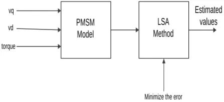
1 (21)The simulation block diagram as shown below;
PMSM Model
LSA Method
Estimated values
Minimize the eror vq
vd
torque
Fig -2: Block diagram of LSA based PMSM
Now in order to apply LS technique for parameter estimation of PMSM motor, it is necessary to write the motor model in the form of model.
Where the Matrix for calculation of eq. (21) is;
r r d ds
q qs
d
i
v
i
v
A
0
0
0
0
0
0
0
0
0
0
© 2015, IRJET ISO 9001:2008 Certified Journal Page
451
r l
e
r l
e
d q
d
T
T
T
T
di
di
Y
02443
.
0
)
(
2
002443
.
0
)
(
2
(23)
d
c
b
a
X
(24)Where
L
a
1
;L
R
b
;j
c
;
d
And dIq is the change in Iq with respect to time.
dId is the change in Id with respect to time.
dωr is the change in ωr with respect to time.
4.2 ALGORITHM:
Step1: Derivation of d-q axes representation of PMSM
equations in rotor reference frame by eliminating immeasurable quantities of damper winding currents at steady state.
Using Least Square Approximation Method on the equations and implementing simulation diagram for estimation of parameters of the modeling equations in MATLAB.
Step2: The simulation of PMSM gives the iqs ,ids and speed. This gives us the information about machine parameters with voltage equations as input.
Step3: the simulation data obtained from simulation of machine is saved and observe the parameters.
Step4: Then obtained Least Square Approximation
Method equations contain machine parameters and are represented in variables.
Step5: By observe the outputs of simulation diagram
calculate the parameters.
Step6: Then note down the results if those are nearer to the true values terminate.
Step7: Otherwise minimize the error and applied to Least
Square Approximation. Then estimated values and true values of machine are compared
Step8: stop
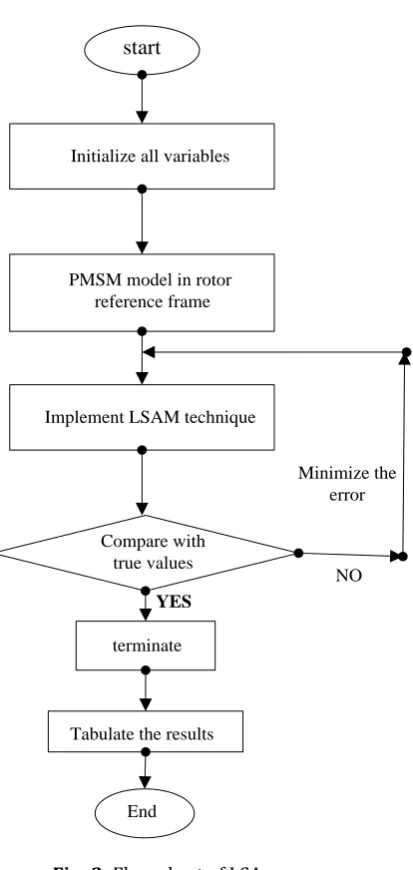
4.3 FLOWCHART:
start
Initialize all variables
PMSM model in rotor reference frame
Implement LSAM technique
Compare with true values
terminate
Tabulate the results
End
Minimize the error
YES
NO
Fig -3: Flow chart of LSA
The above algorithm shows the following method to simulation of PMSM modeling in MATLAB and parameter estimation based on least square approximation. Those steps are involved in flowchart as in diagram.
[image:4.595.355.562.220.656.2]© 2015, IRJET ISO 9001:2008 Certified Journal Page
452
5. RESULT
[image:5.595.33.296.275.433.2]The PMSM motor is modeled as shown in the equations (1) to (11) and simulated in MATLAB or SIMULINK [12] with the assumed parameters which are determined using trial and error method. Then, the algorithm of the Least Squares approximation method, are coded and executed to estimate the parameters of the PMSM motor with the inputs as voltages ,currents, electric torque, load torque, change in currents and speed with respect to time. The actual and estimated parameters of the motor for the PMSM are tabulated below.
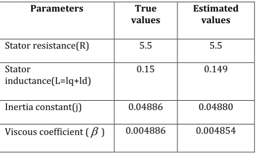
Table -1: Estimated Parameters Using LSA
Parameters True
values
Estimated values
Stator resistance(R) 5.5 5.5
Stator
inductance(L=lq+ld)
0.15 0.149
Inertia constant(j) 0.04886 0.04880
Viscous coefficient (
) 0.004886 0.0048546. CONCLUSION
To achieve goo performance of PMSM has knowledge of machine parameters with more accuracy. In this paper an offline parameter identification of PMSM is done in MATLAB/SIMULINK. The proposed method Least Square Approximation is the one which have less hardware with more accuracy. Firstly the PMSM has modeled in rotor reference frame and implementation of open loop performance of PMSM. Then finding the parameters in LSA method compared with true values which are gathered by classical method
REFERENCES
[1] P. C. Krause, O. Wasynczuk, and S. D. Sudhoff, Analysis of Electric Machinery, IEEE Press, Piscataway, New Jersey, 1996..
[2] P. Pillay and R. Krishnan, Modeling of permanent magnet motor drives, IEEE Trans. Ind. Electron.,35(4), 537–541, 1988.
[3] B. K. Bose, Ed., Power Electronics and Variable Frequency Drives, IEEE Press, Piscataway, New Jersey, 1997, Chapter 6.
[4] Pragasen Pillay and Ramu Krishnan, “Modeling of Permanent Magnet Motor Drives,” IEEE Transactions
on Industrial Electronics, Vol.55, No.4, pp.537-541, November, 1988.
[5] Pragasen Pillay and Ramu Krishnan, “Modeling, simulation and analysis of Permanent Magnet Motor Drives, Part-I: The Permanent Magnet Synchronous Motor Drive,” IEEE Transactions on Industry Applications, Vol.25, No.2, pp.265-273, March/April 1989.
[6] Khwaja M. Rahman and Silva Hiti, ‘Identification of Machine parameters of a Synchronous Motor’, IEEE transactions, 2003
[7] Saab S. S. and Kaed-Bey R. A., “Parameter Identification of a DC Motor: An Experimental Approach,” IEEE International Conf. on Elec. Circuit and Systems. (ICECS),vol.4, pp. 981-984, 2001. [8] Marquardt D. W., “An Algorithm for Least-Squares
Estimation of Nonlinear Parameters,” Journal of the Society for Industrial and Applied Mathematics, vol. 11, No. 2, pp. 431-441, 1963.
[9] Raol J. R., Girija G. and Singh J., “Modeling and
Parameter Estimation of Dynamic Systems”, The Institution of Engineering and Technology, London, United Kingdom Phillips, C. and Nagle, H. 1995.
[10]K.-Y. Wang, J. Chiasson, M. Bodson, and L. M. Tolbert, “A nonlinear least-squares approach for identification of the induction motor parameters,” IEEE Transactions on AutomaticControl, vol. 50, no. 10, pp. 1622–1628, 2005.
[11]A. Zentai and T. Dab´oczi, “Model based torque estimation of permanentmagnet synchronous machines,” in IEEE International Symposiumon Diagnostics for Electric Machines, Power Electronics and Drives, Krakow, Poland, Sept 6–8, 2007, pp. 178– 181.
[12]The Mathworks, Inc., “MATLAB programming language,” 2008, [accessed 15-October-2008]. [Online].
http://www.mathworks.com/products/matlab/ [13] F. Belkhouche, U. Qidwai and B. Belkhouche, “Least