ENHANCED PLANTED(ℓ,D) MOTIF SEARCH PRUNE ALGORITHM FOR PARALLEL ENVIRONMENT

(1)

ISSN: 1992-8645 www.jatit.org E-ISSN: 1817-3195

372

SIMULTANEOUS HYPOTHESIS TESTING OF SPLINE

TRUNCATED MODEL IN NONLINEAR STRUCTURAL

EQUATION MODELING (SEM)

1

RULIANA, 2I.N. BUDIANTARA, B.W.OTOK, W.WIBOWO

1

Department of Statistics, Faculty of Mathematics and Natural Sciences Sepuluh Nopember Institute of Technology (ITS), Surabaya, Indonesia

and

Department of Mathematics, Faculty and Natural Sciences State University of Makassar (UNM), Makassar, Indonesia

2

Department of Statistics, Faculty of Mathematics and Natural Sciences Sepuluh Nopember Institute of Technology (ITS), Surabaya, Indonesia

E-mail: [email protected], [email protected], [email protected],

[email protected]

ABSTRACT

Model of spline truncated in structural equation modeling (SEM) is a nonlinear structural model of SEM that measures a nonlinear relationship between the latent variables. This report was developed a hypothesis testing for the parameter of spline truncated model in nonlinear SEM using likelihood ratio test (LRT). To test hypothesis H :₀ C γ′ =τ versus H :₀ C γ′ ≠τ in spline truncated model of nonlinear SEM for matrix C, vector parameter γ and a constant vector τ, is discovered that a statistical testing is in form of

1 1 2 2

/ /

d d

= Q

W

Q which has a distribution

F d d

( ,

1 2

),

and rejects H0 in which

W values are quite large.

Keywords: Nonlinear SEM, Spline Truncated, Hypothesis Testing, Likelihood Ratio Test

1. INTRODUCTION

Nonlinear SEM is developed from linear SEM studies, which have been previously reported by Joreskog [1], Bentler [2] and Bollen [3]. Several authors have worked about nonlinear SEM in a form of quadratic and interaction such as, Lee and Zhu [4], Lee and Song [5], Lee, Song and Lee [6], Lee, Song and Poon [7], Bollen and Current [8], Lee and Tang [9], Wall and Amemiya [10], Klein and Muthen [11], Mooijaart and Satorra [12]. The nonlinear SEM employing a model of polynomial was investigated by Wall and Amemiya [13], while, model of Griffiths-Miller between latent variable was introduced by Harring [14]. The Bayesian approach in SEM was investigated by Otok, Purnami and Andari [15]. Meanwhile, the current nonlinear structural model SEM using spline truncated was reported by Ruliana, Budiantara, Otok, and Wibowo [16]. Spline truncated model in nonlinear SEM contains knot, which is able to

obtain information in the patterns of relationship between latent variable that keeps changing in particular interval. Some researchers who have especially investigated spline truncated and have published their works are Fernandes, Budiantara, Otok and Suhartono [17], Budiantara [18], Lestari, Budiantara, Sunaryo and Mashuri [19].

In the present study is conducted of hypothesis testing for spline truncated model in nonlinear SEM by applying the likelihood ratio test (LRT).

2. SPLINE TRUNCATED MODEL IN

NONLINEAR STRUCTURAL MODEL SEM

(2)

ISSN: 1992-8645 www.jatit.org E-ISSN: 1817-3195 373 1 1 1 1 1 2 2 2 2 2 1 1 0 1 2 2 0 1 ( ) ( ) m K m r

i r i s i s

r s

m K

m t

t i u i u i

t u

η ξ ξ

ξ ξ

ω α ω β ω κ

α ω β ω κ ζ

+ = = + = = = + − + + + − +

∑

(1)

In matrix form can be formulated as

[ ( , , )]

= +

η ξ1 ξ2

ω T ω ω κ γ ζ (2) where T is the base of functionality that includes exogenous latent variables and knots, which follows previous study [16]. Because of the error

2 ~N( ,

σ

)

ζ 0 I , then

2

( ( , , ) , )

N σ

1 2

η ξ ξ

ω T ω ω κ γ I (3) also

1 2

ˆ

N

( , [ (

′

,

, ) (

,

, )]

−

σ

)

1 2 1 2

ξ ξ ξ ξ

γ

γ T ω

ω

κ T ω

ω

κ

(4)

therefore 1 2 ˆ ( ) ( , [ ( , , , ) ( , , , )] ] ) N σ Ω Ω − ′ − ′ − ′ ′

1 2 1 2

ξ ξ 1 2 ξ ξ 1 2

C γ τ C γ τ

C T ω ω κ κ T ω ω κ κ C

(5) to determine whether parameters

1 1

2 2

10 11 1 11 1

20 21 2 21 2

[ , , , , , , ,

, , , , , , , ]

m K

α α α β β

=

′

γ K K

K K

influence model in Eq.(1), we will conduct hypothesis testing for H :0 C γ′ =τ versus

1

H :C γ′ ≠τ.

3. PARAMETER ESTIMATION UNDER SPACE Ω AND SPACE Ψ_{OF SPLINE} TRUNCATED IN NONLINEAR

STRUCTURAL MODEL SEM

Parameter hypothetical test for model (1) as expressed below

0

H :C γ′ =τ versus H :₁ C γ′ ≠τ (6) where C′ is matrix s d× 1,

1 1 2 1 2 2

d =m +m +k +k + , γ is d₁×1 vector parameter and τ is vector s×1 that the elements are constant. Parameters set under population, or under the parameter space Ω is as follows:

1 1

2 2

10 11 1 11 1 2 20 21 2 21 2

{ ( , , , , , , ,

, , , , , , , ), }

m K

m K ωη

α α α β β

α α α β β σ _Ω

Ω = γ= K K

K K (7)

The set of parameters under H₀ or parameter space

Ψ are formulated as follows:

1 1

2 2

10 11 1 11 1 2 20 21 2 21 2

{ ( , , , , , , ,

, , , , , , ), }

m K

m K ω_η

α α α β β

α α α β β σ _Ψ

Ψ = =

′ = γ

C γ τ

K K K K (8) with 1r

α

−∞ < < ∞ ; r=0,1,...,m1

2t

α

−∞ < < ∞ ; t=0,1,...,m₂

1s

β

−∞ < < ∞ ; s=1, 2,...,K₁

2u

β

−∞ < < ∞ ; u=1, 2,...,K₂

and

2

0<

σ

_ω_η_Ω < ∞; 0<

σ

_ω2_η_Ψ < ∞

To obtain the parameter estimation of γ in the parameter space Ω and parameter space Ψ for model (1), are available in the following lemma:

Lemma 1

If γˆ_Ω and γˆ_Ψ are estimators of γ under space Ω and Ψ for model (1), respectively, then:

1

1 1

ˆ ˆ [ ( , , , ) ( , , , )]

[ [ ( , , , ) ( , , , )] ] ˆ ( ) − Ψ Ω − − Ω ′ = − ′ ′ × ′ × −

1 2 1 2

ξ ξ 1 2 ξ ξ 1 2

γ γ T ω ω κ κ T ω ω κ κ C

C T ω ω κ κ T ω ω κ κ C

C γ τ

Proof

To prove Lemma 1 as described above can be used Lagrange multipliers’s method. The Lagrange function is assumed the following:

F(γ_Ψ, )θ =V(γ_Ψ) 2 (+ θ C γ′ ′ _Ψ−τ) (9) where

V( ) [( ( , , ) )

( ( , , ) ] Ψ Ψ Ψ ′ = − × − 1 2 1 2

η ξ ξ

γ ω T ω ω κ γ

ω T ω ω κ γ

(10) and 2θ′ is Lagrange multipliers vector. Estimation of γ_Ψ is γˆ_Ψ which minimizes an equation in form of:

ˆ ˆ

V( ) [( ( , , ) )

ˆ ( ( , , ) ] Ψ Ψ Ψ ′ = − × − 1 2 1 2

η ξ ξ

γ ω T ω ω κ γ

ω T ω ω κ γ

(11) with constrain of C γ′ˆ_Ψ =τ. Estimator of γˆ_Ψ is obtained by describing the Eq.(10) to be

V( ) 2 ( , , , )

( , , , ) ( , , , ) Ψ Ψ Ψ Ψ ′ ′ ′ = − + ′ ′ + 1 2

1 2 1 2

η η ξ ξ 1 2 η

ξ ξ 1 2 ξ ξ 1 2

γ ω ω γ T ω ω κ κ ω

γ T ω ω κ κ T ω ω κ κ γ

(12) By substituting Eq.(12) into Eq.(9), it generates an

equation

F( , ) 2 ( , , , )

( , , , ) ( , , , )

2 ( )

Ψ Ψ Ψ Ψ Ψ ′ ′ ′ = − + ′ ′ + + ′ ′ + − 1 2

1 2 1 2

η η ξ ξ 1 2 η

ξ ξ 1 2 ξ ξ 1 2

γ θ ω ω γ T ω ω κ κ ω

γ T ω ω κ κ T ω ω κ κ γ

θ C γ τ

(13) When the Eq.(13) is derived with respect to γ_Ψ and

(3)

374 F( , )

2 ( , , , )

2 ( , , , ) ( , , , ) 2

Ψ Ψ Ψ ∂ _′ =− + ∂ ′ + + 1 2

1 2 1 2

ξ ξ 1 2 η

ξ ξ 1 2 ξ ξ 1 2

γ θ

T ω ω κ κ ω γ

T ω ω κ κ T ω ω κ κ γ Cθ

(14) For the Eq.(14) is minimized, it is equal to zero and then by carrying out a simplification, it yields:

2 ( , , , ) 2 ( , , , )

ˆ

( , , , ) _Ψ 2

′ ′

− +

× + =

1 2 1 2

1 2

ξ ξ 1 2 η ξ ξ 1 2

ξ ξ 1 2

T ω ω κ κ ω T ω ω κ κ

T ω ω κ κ γ Cθ 0

1

ˆ [ ( , , , ) ( , , , )]

[ ( , , , ) ]

−

Ψ = ′

′

× −

1 2 1 2

1 2

ξ ξ 1 2 ξ ξ 1 2

ξ ξ 1 2 η

γ T ω ω κ κ T ω ω κ κ

T ω ω κ κ ω Cθ

1

ˆ

_Ω

[ (

′

,

, ,

) (

,

, ,

)]

−

=

−

1 2 1 2

ξ ξ 1 2 ξ ξ 1 2

γ T ω ω κ κ T ω ω κ κ Cθ (15) And by deriving the Eq.(13) with respect to θ and

treat the result equals to zero; it yields a form F( , )

2 2 Ψ Ψ ∂ ′ = − ∂ γ θ

C γ τ

θ

(16) ˆ_Ψ

′ =

C γ τ

(17) By substituting Eq.(15) into Eq.(17), it generates an equation

ˆ_Ω [ ( , , , ) ( , , , ) ]

′ − ′ ′ =

1 2 1 2

ξ ξ 1 2 ξ ξ 1 2

C γ C T ω ω κ κ T ω ω κ κ Cθ τ

Then by adding the both sides with vector C γ′ˆ_Ω generates a compiled equation

1

_ˆ

[ [ (

′ ′

,

, , ) (

,

, , )]

−

] (

=

′

_Ω

−

)

1 2 1 2

ξ ξ 1 2 ξ ξ 1 2

C T ω ω κ κ T ω ω κ κ Cθ Cγ τ

1

_ˆ

[

′ ′

(

,

, , ) (

,

, , ) ] (

−

′

_Ω

)

=

−

1 2 1 2

ξ ξ 1 2 ξ ξ 1 2

θ CT ω ω κ κ T ω ω κ κ C Cγ τ

(18) And by substituting the Eq. (18) into Eq. (15), is yielded:

1 1 1

ˆ ˆ [ ( , , , ) ( , , , )]

[ [ ( , , , ) ( , , , )] ] ˆ ( ) − Ψ Ω − − Ω ′ = − ′ ′ × ′ × −

1 2 1 2

ξ ξ 1 2 ξ ξ 1 2

γ γ T ω ω κ κ T ω ω κ κ C

C T ω ω κ κ T ω ω κ κ C

C γ τ

(19) Based on Eq.(19) as previously described, the Lemma 1 is proved.

4. STATISTICAL TEST OF SPLINE TRUNCATED IN NON LINEAR SEM

Statistical test for hypothesis testing parameter in the Eq.(6) by using likelihood ratio test is given into Theorem 1 the following :

Theorem 1

The spline truncated model in nonlinear SEM is given such as the Eq.(1) If the hypothesis in the Eq.(6) is tested, then the statistical test for this hypothesis is: 1 1 2 2 / / d d = Q W Q , where

1 1 2 1 2 2

d =m +m +k +k +

2 ( 1 2 1 2 2)

d = −n m +m +k +k +

1 1

1 ( ˆ ) [ [ ( , , , ) ( , , , )] ]

ˆ ( ) − − Ω Ω ′ ′ ′ ′ = − ′ × −

1 2 1 2

ξ ξ 1 2 ξ ξ 1 2

Q C γ τ C T ω ω κ κ T ω ω κ κ C

C γ τ

2=[ η− ( ξ₁, ξ₂, )ˆΩ] [′ η− ( ξ₁, ξ₂, )ˆΩ]

Q ω T ω ω κ γ ω T ω ω κ γ

Proof

The Theorem 1 can be tested by employing a likelihood ratio test (LRT). Core method of LRT is purposed at searching for ratio results from the likelihood function which is the maximum value under parameter space of Ψ against the likelihood function which is the maximum value under parameter space Ω. By using parameter sets of space Ω and space Ψ in the Eq.(7) and (8) respectively, can be written likelihood function for model (1) under Ω as follows:

2 2 / 2

2

1

( , ) (2 ) exp{ [

2

2 ( , , )

( , , ) ( , , ) ]}

n

L _η _η

η ω ω ω σ πσ σ −

Ω Ω Ω

Ω Ω Ω Ω ′ = − + ′ ′ − + ′ ′ + 1 2

1 2 1 2

η η

ξ ξ η

ξ ξ ξ ξ

γ ω ω

γ T ω ω κ ω

γ T ω ω κ T ω ω κ γ

(20)

If the logarithm of the Eq.(20) is derived partially with respect to 2

η ω

σ

_Ω and make the result equals to zero then it is obtained:

2 ( ( , , )ˆ ) ( ( , , )ˆ )

ˆ

n

η

ω

σ _Ω= ωη−T ωξ1 ωξ2 κ γΩ ′ωη−T ωξ1 ωξ2 κ γΩ

(21) Authors, Ruliana et al (2015), showed that the estimator for

γ

under the space Ω was

1

ˆ [ ( , , ) ( , , )]

( , , )

−

Ω = ′

′ ×

1 2 1 2

1 2

ξ ξ ξ ξ

ξ ξ η

γ T ω ω κ T ω ω κ

T ω ω κ ω (22)

It is discovered that by using Eq.(22) and Eq.(21) the maximum value of likelihood function under parameter space Ω_{is yielded:}

2 2 / 2 /2

ˆ _ˆ _ˆ _ˆ

( ) ( , ) (2 ) n e n

L Ω =L γΩ

σ

_ω_ηΩ =

πσ

_ω_ηΩ − − (23)

Subsequently, the likelihood function model (1) under the space Ψ is:

2 2 /2

2

1

( , ) (2 ) exp{ (

2

2 ( , , )

( , , ) ( , , ) )}

n

L _η _η

η ω ω ω σ πσ σ −

Ψ Ψ Ψ

Ψ Ψ Ψ Ψ ′ = − + ′ ′ − + ′ ′ + 1 2

1 2 1 2

η η

ξ ξ η

ξ ξ ξ ξ

γ ω ω

γ T ω ω κ ω

(4)

375 (24)

By partially deriving the logarithm of Eq. (24), with respect to 2

η ω

σ

_Ψ and make the result equals to zero, it is resulted:

2 ( ( , , ) )'( ( , , ) )

ˆ

n

η

ω

σ Ψ Ψ Ψ

− −

= ωη T ω ωξ1 ξ2 κ γ ωη T ω ωξ1 ξ2 κ γ

(25) and based on Lemma 1, the mathematical form is obtained the following:

1 1 1

ˆ ˆ [ ( , , , ) ( , , , )]

[ [ ( , , , ) ( , , , )] ] ˆ ( ) − Ψ Ω − − Ω ′ = − ′ ′ × ′ × −

1 2 1 2

ξ ξ 1 2 ξ ξ 1 2

γ γ T ω ω κ κ T ω ω κ κ C

C T ω ω κ κ T ω ω κ κ C

C γ τ

by applying Eq.(19) and Eq.(25), maximum value of likelihood function under parameter space Ψ is yielded

2 2 / 2 /2

ˆ _ˆ _ˆ _ˆ

( ) ( , ) (2 ) n e n

L Ψ =L γ_ω

σ

_ω_ηΨ =

πσ

_ω_ηΨ − − (26)

Subsequently, by dividing of Eq.(26) toward Eq.(23) likelihood ratio is resulted as follows:

2 / 2 / 2 ratio 2 / 2 / 2

(2 )

ˆ ( ) L

ˆ ₍₂ ₎

( ) n n n n e L e L η η ω ω πσ πσ − − Ψ − − Ω Ψ = = Ω 2 2 n  

= _Q _

A (27)

where

ˆ ˆ

( ( , , ) _Ψ) '( ( , , ) _Ψ)

= − −

1 2 1 2

η ξ ξ η ξ ξ

A ω T ω ω κ γ ω T ω ω κ γ

(28)

2=( η− ( ξ1, ξ2, )ˆΩ) (′ η− ( ξ1, ξ2, )ˆΩ)

Q ω T ω ω κ γ ω T ω ω κ γ

(29) By elaborating Eq. (28) the form _Acan be written as follows: ˆ ( ( , , ) ) ˆ ( ( , , ) ) Ψ Ψ ′ = − × − 1 2 1 2

η ξ ξ

A ω T ω ω κ γ

ω T ω ω κ γ

ˆ ˆ

[[ ( , , ) ] ( ( , , ) ]

ˆ ˆ ˆ

[( ( , , ) ] ( , , )( )]

ˆ ˆ ˆ

( ) ( , , )( ( , , )

ˆ ˆ ˆ ˆ

( ) , , ) ( , , )( )

Ω Ω

Ω Ω Ψ

Ω Ψ Ω

Ω Ψ Ω Ψ

′ = − − + ′ + − − + ′ ′ + − − + ′ ′ + − −

1 2 1 2

η ξ ξ η ξ ξ

η ξ ξ ξ ξ

ξ ξ η ξ ξ

ξ ξ ξ ξ

ω T ω ω κ γ ω T ω ω κ γ

ω T ω ω κ γ T ω ω κ γ γ

γ γ T ω ω κ ω T ω ω κ γ

γ γ T ω ω κ T ω ω κ γ γ

(30) Because of

ˆ

[( − ( , , ) _Ω]′ ( , , )=

1 2 1 2

η ξ ξ ξ ξ

ω T ω ω κ γ T ω ω κ 0

ˆ

( , , )[ ( , , ) _Ω]

′ − =

1 2 1 2

ξ ξ η ξ ξ

T ω ω κ ω T ω ω κ γ 0

and

1

[ (

′

,

, ) (

,

, )]

−

′

(

,

, ) (

,

, )

=

1 2 1 2 1 2 1 2

ξ ξ ξ ξ ξ ξ ξ ξ

T ω ω κ T ω ω κ T ω ω κ T ω ω κ I

then Eq. (30) can be formulated to be

ˆ ˆ

( ( , , ) ) ( ( , , ) )

ˆ ˆ ˆ ˆ

( ) , , ) ( , , )( )

Ω Ω

Ω Ψ Ω Ψ

′

= − − +

′ ′

+ − −

1 2 1 2

η ξ ξ η ξ ξ

ξ ξ ξ ξ

A ω T ω ω κ γ ω T ω ω κ γ

γ γ T ω ω κ T ω ω κ γ γ

(31) Eq. (31) including previous Eq.(19) while the

Eq.(19) can be decomposed into

1

1 1

ˆ ˆ [ ( , , , ) ( , , , )]

[ [ ( , , , ) ( , , , )] ] ˆ ( ) − Ω Ψ − − Ω ′ − = ′ ′ × ′ × −

1 2 1 2

ξ ξ 1 2 ξ ξ 1 2

γ γ T ω ω κ κ T ω ω κ κ C

C T ω ω κ κ T ω ω κ κ C

C γ τ

(32) So, by substituting the Eq.(32) into Eq.(31)

expression of A becomes

1 1 ˆ ( ( , , ) ) ˆ ˆ ( ( , , ) ) ( ) [ [ ( , , , ) ( , , , )] ] ˆ ( ) Ω Ω Ω − − Ω ′ = − ′ ′ × − − ′ ′ × ′ × − 1 2 1 2

1 2 1 2

η ξ ξ

ξ ξ 1 2 ξ ξ 1 2

A ω T ω ω κ γ

ω T ω ω κ γ C γ τ

C T ω ω κ κ T ω ω κ κ C

C γ τ

=Q₂+Q₁ (33) where 1 1 1 ˆ ( ) [ [ ( , , , ) ( , , , )] ] ˆ ( ) Ω − − Ω ′ ′ = − ′ ′ × ′ × −

1 2 1 2

ξ ξ 1 2 ξ ξ 1 2

Q C γ τ

C T ω ω κ κ T ω ω κ κ C

C γ τ

(34) Then by substituting the Eq.(33) into Eq.(27) and elaborating the likelihood ratio, the Eq.(27) can be written as follows:

/ 2 1 ratio 2 L 1 n −   =_ + _   Q

Q

(35)

Based on the Eq.(35), and conducted a slightly elaboration , it is obtained that the statistical test for hypothesis H :₀ C γ′ =τ versus H :₀ C γ′ ≠τ from model of (1) is expressed in form of

1 1 2 2 / / d d = Q W Q

5. DISTRIBUTION OF STATISTICAL TEST AND CRITICAL AREA OF HYPOTHESIS PARAMETER FOR SPLINE TRUNCATED MODEL IN NONLINEAR SEM

The distribution from statistical test resulted by Theorem 1 is derived and is written in Theorem 2 as follows:

Theorem 2

(5)

ISSN: 1992-8645 www.jatit.org E-ISSN: 1817-3195 376 1 1 1 2 2 2 / ( , ) / d

F d d d

= Q

W Q

Proof

To prove the Theorem 2, should be shows

2 2 1/σ (d1)

Q χ , Q₂/σ2 χ2(d₂), also Q₁ and

2

Q are independent, with the description is stated below as follows:

From Eq.(34) with

1 2 ˆ ( ) ( , [ ( , , , ) ( , , , )] ] ) N σ Ω Ω − ′ − ′ − ′ ′ × 1 2 1 2

ξ ξ 1 2

C γ τ C γ τ C T ω ω κ κ

T ω ω κ κ C

and (AV) (′ AV)=(AV) is an idempotent matrix where 1 1 2 [ [ ( , , , ) ( , , , )] ] σ − − ′ ′

= C T ωξ1 ωξ2 κ κ T ω1 2 ξ1 ωξ2 κ κ1 2 C

A

2 1

[ [ ( , , , ) ( , , , )] ]

σ _{′ ′} −

=

1 2 1 2

ξ ξ 1 2 ξ ξ 1 2

V C T ω ω κ κ T ω ω κ κ C

then

2 1

2 (rank( ), )

σ Q

χ A D (36) with 1 1 2 ( ) [ [ ( , , , ) ( ) ( , , , )] ] 2σ Ω

− − Ω

′ ′ ′ ′ = − ′ − × 1 2 1 2

ξ ξ 1 2

D C γ τ C T ω ω κ κ

C γ τ

T ω ω κ κ C

Since A is the full rank matrix with the order d1 and it is under the hypothesis H₀, also matrix D=0, then the form of Eq.(36) becomes

2 1

1 2 ( )d

σ

Q

χ (37)

Moreover, to show that Q₂/σ2 χ2(d₂) it was conducted a modification of Eq.(29) into the form of quadratic form with the following description:

2 [ ( , , )ˆ ]

ˆ [( ( , , ) )] Ω Ω ′ = − × − 1 2 1 2

η ξ ξ

Q ω T ω ω κ γ

ω T ω ω κ γ

=ω′_η[J J ω] _η (38) where 1 [ ( , , )[ ( , , ) ( , , )] ( , , )] − ′ = − ′ ×

1 2 1 2 1 2

1 2

ξ ξ ξ ξ ξ ξ

ξ ξ

J I T ω ω κ T ω ω κ T ω ω κ

T ω ω κ

For J J′ =J is symmetric and idempotent matrix, then the form of Eq.(38) can be rewritten as follows:

1

2 [ ( , , )[ ( , , ) ( , , )]

( , , )] − ′ ′ = − ′ ×

1 2 1 2 1 2

1 2

η ξ ξ ξ ξ ξ ξ

ξ ξ η

Q ω I T ω ω κ T ω ω κ T ω ω κ

T ω ω κ ω

(39)

with N( ( , , ) ,σ2 )

1 2

η ξ ξ

ω T ω ω κ γ I

and (A V_{∗ ∗}) (′ A V_{∗ ∗})=(A V_{∗ ∗}) is idempotent matrix where 1 2 [ ( , , )[ ( , , ) ( , , )] ( , , ) σ − ∗ ′ ′ −

= I T ωξ1 ωξ2 κ T ωξ1 ωξ2 κ T ωξ1 ωξ2 κ T ωξ1 ωξ2 κ

A

2

σ

∗=

V I

Then it is obtained the following

2 2

2 (rank( ), )

σ ∗

Q

χ A E (40)

with 1 2 ( ( , , ) ) [ ( , , ) [ ( , , ) ( , , )] ( ( , , ) ) ( , , ) 2σ − ′ = − ′ × ′ ×

1 2 1 2

1 2

ξ ξ ξ ξ

ξ ξ

E T ω ω κ γ I T ω ω κ

T ω ω κ T ω ω κ

T ω ω κ γ

T ω ω κ

since

1 2 1 2

rank( ) rank( ) tr( )

( 2)

n m m k k

∗ ∗

= =

= − + + + +

A A V

AV

and by elaborating the matrix E, it is yielded that

=

E 0, then Eq.(40) becomes into

2

2 2 (d )

σ

2

Q

χ (41)

Furthermore, to show whether Q₁ and Q₂

are independent or not, it should be shown

=

GVF 0, where V=σ2I is the variance of vector quadratic form Q₁ and Q₂; G and F, respectively, are matrix quadratic form for Q₁and Q₂. By modifying Q₁ in the Eq.(34) and Q₂ in the Eq.(29) into vector quadratic form as random variable distributed normally, Q₁ and Q₂ respectively are obtained in form of:

1 1 1 1 1 1 [ ( , , ) [ ] ] ( , , )[ ( , , ) ( , , )] [ [ ( , , , ) ( , , , )] ] [[ ( , , ) ( , , )] ( , , ) − − − − − ′ ′ = − ′ × ′ ′ × ′ ′ ′ × 1 2

1 2 1 2 1 2

1 2 1 2

1 2 1 2 1 2

η ξ ξ

ξ ξ ξ ξ ξ ξ

ξ ξ 1 2 ξ ξ 1 2

ξ ξ ξ ξ ξ ξ

Q ω T ω ω κ C C C τ

T ω ω κ T ω ω κ T ω ω κ C

C T ω ω κ κ T ω ω κ κ C

C T ω ω κ T ω ω κ T ω ω κ

×

[

−

(

,

, ) [

′

]

−1

]

1 2

η ξ ξ

ω T ω ω κ C C C τ (42)

and 1 2 1 1 [ ( , , ) [ ] ] [ ( , , )[ ( , , ) ( , , )] ( , , )][ ( , , ) [ ] ] − − − ′ ′ = − ′ × − ′ ′ × − 1 2

1 2 1 2 1 2

1 2 1 2

η ξ ξ

ξ ξ ξ ξ ξ ξ

ξ ξ η ξ ξ

Q ω T ω ω κ C C C τ

I T ω ω κ T ω ω κ T ω ω κ

T ω ω κ ω T ω ω κ C C C τ

(6)

377 From the Eq.(42) and Eq.(43) are found that Q₁

and Q₂ are quadratic form in vector

1

[

(

,

, ) [

′

]

−

]

=

−

1 2

η ξ ξ

x ω T ω ω κ C C C τ distributed

normally, where matrix quadratic form for Q₁ is:

1

1 1

( , , )[ ( , , ) ( , , )]

[ [ ( , , , ) ( , , , )] ]

−

− −

′ =

′ ′ ×

1 2 1 2 1 2

1 2 1 2

ξ ξ ξ ξ ξ ξ

ξ ξ 1 2 ξ ξ 1 2

F T ω ω κ T ω ω κ T ω ω κ C

C T ω ω κ κ T ω ω κ κ C

1

[[ (

,

, ) (

,

, )]

−

(

,

, )

′ ′

′

×

1 2 1 2 1 2

ξ ξ ξ ξ ξ ξ

C T ω ω κ T ω ω κ T ω ω κ

(44) and matrix quadratic form for Q₂ is:

1

[

(

,

, )[ (

,

, ) (

,

, )]

(

,

, )

−

′

= −

′

×

1 2 1 2 1 2

1 2

ξ ξ ξ ξ ξ ξ

ξ ξ

G

I T ω ω

κ T ω ω κ T ω ω κ

T ω ω κ

(45) By using the results of the multiplication of the matrices in Eq.(45) and Eq.(44) also variance from

1

[

ωη

−

T ω

(

ξ₁

,

ωξ₂

, ) [

κ C C C

′

]

− τ

]

, slightly Elaboration obtained:

2 2

(

σ

)

σ

= = =

GVF G I F

GF 0

(46)

It results that Q₁ and Q₂ are independent. Based on the Eq.(37), Eq.(41) and Eq.(46) then the form of distribution from statistical test of spline truncated in nonlinear SEM in the equation of (1) is:

1 1

1 2 2 2

/

( , )

/

d

F d d d

= Q

W

Q

The critical area of hypothesis of statistical test for spline truncated model in nonlinear SEM is described in Theorem 3 as follows:

Theorem 3

If given a hypothesis such as in Eq.(6), and statistical test as stated in Theorem 1 as well as the distribution of the statistical test, which is given by Theorem 2, then the critical areas of the test are obtained from completing the equation:

(

)

P W>k∗ Cγ=τ =α

where α and

k

∗ are the significant level and a particular constant, respectively.

Proof

The critical area to test hypothesis H :₀ C γ′ =τ

versus H :₁ C γ′ ≠τ, is the sets of all points that satisfy the condition

ratio

ˆ ( ) L

k L

Ψ

= <

Ω (47)

or

2

(1 )

n k

−

+Q < (48) By decomposing the expression of inequality stated in Eq.(48) is obtained

k > ∗

W (49)

where

2 2 1

1

n d k k

d

−

 

 

∗ = −

 

 

Then if given a significant level of α then

k

∗ is resulted from the equation of shown below:

(

)

P k

α₌ _> ∗ ₌

W Cγ τ , where W F d d( ,₁ ₂)

6. CONCLUSION

Hypothesis testing of parameter of spline truncated model in nonlinear SEM for

0

H :C γ′ =τ versus H :₁ C γ′ ≠τ using Likelihood Ratio Test (LRT), can be concluded as follows:

1. Estimation of parameter for spline truncated model in nonlinear SEM under parameter space Ω is:

1

ˆ

_Ω

=

[ (

′

ξ₁

,

ξ₂

, ) (

ξ₁

,

ξ₂

, )]

−

′

(

ξ₁

,

ξ₂

, )

η

γ T ω ω κ T ω ω κ T ω ω κ ω

and under parameter space Ψ(hypothesis H0) is:

1

1 1

ˆ ˆ [ ( , , , ) ( , , , )]

[ [ ( , , , ) ( , , , )] ]

ˆ

( )

−

Ψ Ω

− −

Ω

′

= −

′ ′ ×

′

× −

1 2 1 2

ξ ξ 1 2 ξ ξ 1 2

γ γ T ω ω κ κ T ω ω κ κ

C C T ω ω κ κ T ω ω κ κ C

C γ τ

2. Statistical test for hypothesis test of parameter for spline truncated model in nonlinear SEM is:

1 1

2 2

/ /

d d

= Q

W Q where

d₁=m₁+m₂+k₁+k₂+2 d₂ = −n (m₁+m₂+k₁+k₂+2)

1

1 1

ˆ

( )

[ [ ( , , , ) ( , , , )] ]

ˆ

( )

Ω

− −

Ω

′ ′

= −

′ ′ ×

′

× −

1 2 1 2

ξ ξ 1 2 ξ ξ 1 2

Q Cγ τ

C T ω ω κ κ T ω ω κ κ C

Cγ τ

2 ( ( , , )ˆ )

ˆ

( ( , , ) )

Ω

′

= −

× −

1 2

η ξ ξ

Q ω T ω ω κ γ

(7)

378 3. Distribution of statistical test for hypothesis

testing of parameter for spline truncated model in nonlinear SEM is in form of: W F d d( ,₁ ₂)

4. Critical area for hypothesis test of parameter for spline truncated model in nonlinear SEM is obtained from the solving of equation

P

(

W>k∗ Cγ=τ

)

=α,where W F d d( ,₁ ₂)

REFERENCES

[1] K.G. Joreskog, A General Method for Estimating a Linear Structural Equation System, in A.S. Goldberger, O.D. Duncan, (Eds.), Structural Equation Models in the Social Sciences 85-112, Academic Press, New York, 1973.

[2] P.M. Bentler, Multivariate Analysis with Latent Variables: Causal Modeling, Annual Review of Psychology, Vol. 31, 1980, pp. 419-456. http://dx.doi.org/10.1146/annurev.ps.31.02018 0.002223

[3] K.A. Bollen, Structural Equations with Latent Variables, John Wiley & Sons, New York, 1989.

http://dx.doi.org/10.1002/9781118619179 [4] M.M. Wall, and Y. Amemiya, Nonlinear

Structural Equation Modeling as a Statistical Method, Handbook of Computing and Statistics With Applications, ISSN: 1871-0301 Vol. 1, 2007, pp. 321-343.

http://dx.doi.org/10.1016/b978-044452044-9/50018-5

[5] S.Y. Lee, and H.T. Zhu, Statistical Analysis of Nonlinear Structural Equation Models with Continuous and Polytomous Data, British Journal of Mathematical and Statistical Psychology, Vol. 53, 2000, pp. 209-232. http://dx.doi.org/10.1348/000711000159303 [6] S.Y. Lee, and X.Y. Song, Maximum Likelihood

Estimation and Model Comparison of Nonlinear Structural Equation Models with Continuous and Polytomous Variables,

Computational Statistics & Data Analysis,

Vol. 44, 2003, pp. 125-142.

http://dx.doi.org/10.1016/s0167-9473(02)00305-5

[7] S.Y. Lee, X.Y. Song and J.C.K. Lee, Maximum Likelihood Estimation of Nonlinear Structural Equation Models with Ignorable Missing Data, Journal of Educational and Behavioral Statistics, Vol. 28, 2003, pp. 111-134. http://dx.doi.org/10.3102/1076998602800211 1

[8] S.Y. Lee, X.Y. Song, and W.Y. Poon, Comparison of Approaches in Estimating Interaction and Quadratic Effects of Latent Variables, Multivariate Behavioral Research, Vol. 39, 2004, pp. 37-67.

http://dx.doi.org/10.1207/s15327906mbr3901 _2

[9] K.A. Bollen, and P.J. Curran, Non Linear Trajectories and The Coding of Time, Latent Curve Models: a Structural Equation Perspective, John Wiley & Sons, 2006. [10] S.Y. Lee, and N.S. Tang, Analysis of

Nonlinear Structural Equation Models with Nonignorable Missing Covariates and Ordered Categorical Data, Statistica Sinica, Vol. 16, 2006, pp. 1117-1141.

[11] A.G. Klein, and B.O Muthen, Quasi Maximum Likelihood Estimation of Structural Equation Models with Multiple Interaction and Quadratic Effects, Multivariate Behavioral

Research, Vol. 42, 2007, pp. 647-673. http://dx.doi.org/10.1080/0027317070171020 5

[12] A. Mooijaart, and A. Satorra, Moment Testing for Interaction Terms in Structural Equation Modeling, Leiden University, 2011.

[13] M.M. Wall, and Y. Amemiya, Estimation for Polynomial Structural Equation Models,

Journal of the American Statistical Association, Vol. 9, 2000, pp. 929-940. http://dx.doi.org/10.1080/01621459.2000.104 74283

[14] J.R. Harring, a Spline Model for Latent Variable, Educational and Psychological Measurement, Vol. 20,2013, pp. 1-7.

[15] B.W. Otok, S.W. Purnami, and S. Andari, Developing Measurement Model Using Bayesian Confirmatory Factor Analysis in Suppressing Maternal Mortality, International Journal of Applied Mathematics and Statistics, Vol. 6, 2015, pp. 130-136.

[16] Ruliana, I.N. Budiantara, B.W. Otok and W.Wibowo, Parameter Estimation of Nonlinear Structural Model SEM Using Spline Approach, Applied Mathematical Sciences, Vol. 9, 2015, pp. 7439-7451. http://dx.doi.org/10.12988/ams.2015.510660 [17] A.A.R. Fernandes, I.N. Budiantara, B.W. Otok

and Suhartono, Spline Estimator for Bi-responses Nonparametric Regression Model for Longitudinal Data, Applied Mathematical Sciences, Vol.8, 2014, pp. 5653-5665.

(8)

379 [19] B. Lestari, I.N. Budiantara, S. Sunaryo, and M.

Mashury, Spline Estimator in Multiresponses Nonparametric Regression Model with Unequal Correlation of Errors, Mathematics and Statistics, Vol. 6, No. 3, 2010, pp. 327-332

(9)

380

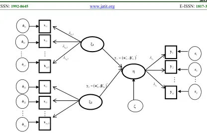
ζ ξ1

ξ2

[image:9.612.93.509.69.337.2]

η

Figure 1: Path Diagram of Spline Truncated Model in Nonlinear SEM for Two Exogenous Latent Variables and One Endogenous Latent