RECOGNITION AND LOCALIZATION OF HARMFUL
ACOUSTIC SIGNALS IN WIRELESS SENSOR NETWORK
BASED ON ARTIFICIAL FISH SWARM ALGORITHM
ZONGZHANG LI, HAIXIA ZHANG*, JIALI XU AND QINGYU ZHAI
School of Information Science and Engineering, Shandong University, Jinan250100, China
*
Corresponding authorE-mail: [email protected], [email protected]
ABSTRACT
The recognition and localization of harmful acoustic signals in a certain scenario are of great importance. In this paper, we propose a scheme for harmful acoustic signals recognition and localization based on fish swarm algorithm for wireless sensor network. We firstly optimize the coverage where the harmful sound source can be detected efficiently. And then, we get the eigenvalue of the harmful acoustic signals by using the LPC (Linear Prediction Coefficients). After analyzing the similarity between the eigenvalue and the data pre-stored in the data base, we can find out the harmful sound. After detection, the harmful resource is located with the help of its closest nodes which are chosen based on time delay. Simulation results show that the proposed scheme can improve the efficiency of harmful source detection and accuracy of the localization.
Keywords: Artificial fish swarm algorithm; Harmful acoustic signals; Linear Prediction Coefficients; Recognition; Localization
1. INTRODUCTION
Artificial fish-swarm algorithm is a new kind of cluster intelligent optimization algorithm. It was first proposed in [1] for system optimization and has been applied in route selection in computer networks and feed-forward neural networks [2, 3]. At present, the nodes arrangement for wireless sensor network by artificial fish-swarm algorithm has become quite mature. But those related researches focus only on coverage arrangement of the sensor nodes and pays no attention on further applications [4]. On the other hand, the study on recognition and localization of harmful acoustic signals in a certain scenario is also very popular duing the past years but far from perfect. For instance, [5] concentrates only on the recognition and localization of harmful acoustic signals but do nothing on the arrangement of the sensor nodes. It is still an open problem how to joint consider the coverage of sensor networks and the recognition and localization of harmful acoustics. Focusing on this, we proposed a scheme for harmful acoustic signals recognition and localization based on fish swarm algorithm for wireless sensor network. To fulfill this, we firstly optimize the coverage where the harmful sound source can be detected
efficiently. And then, we get the eigenvalue of the harmful acoustic signals by using the LPC. After analyzing the similarity between the eigenvalue and the data pre-stored in the data base, we can locate the source. Simulation results show that the proposed scheme can improve the efficiency of the harmful source detection and the accuracy of the localization.
The remainder of the paper is organized as follows. Sec.2 develops the system model of the wireless sensor network based on the artificial fish-swarm algorithm. In Sec.3, LPC is applied to recognize the harmful acoustic signals and decide the time difference of arrival technology(TDOA) to localize the sound source. And finally inSec.4, simulation results are presented. Sec.5 analyzes the results and Sec. 6 concludes the whole paper.
2. WIRELESS SENSOR NETWORK BASED
ON THE ARTIFICIAL FISH ALGORITHM
nodes is large enough. To be clear, we list the characteristic of the sensor nodes as follows:
a) The sensor network is dynamic. Namely, the node can be moved
b) The initial positions of the sensor nodes are generated randomly, and their coordinates are known.
c) The perception radius of each node is r ; And the communication region is a spherical area with the radius of r .
d) The model and the physical structure of each node are same
Therefore, the model featured in this part can be concluded as follows: all the
N
sensor nodes are given and their coordinates will be determined randomly to set up a working set of nodes which is named C1. A working set of nodes C2 need to be set up by moving the sensor nodes to ensure that the network coverage could meet the predefined demands after the optimization with the artificial fish-swarm algorithm.2.2 The Artificial Fish-Swarm Algorithm And Realization Of The Model
The basic idea of artificial fish-swarm algorithm is elaborated as follows. Since fishes can always find the position full of nutrition by themselves or by following the other fishes, thus the space with the most survival is usually the place that offers the most nutrients. Considering this characteristic, artificial fish algorithm optimizes systems by simulating all kinds of fish actions and combines them with animals’ body model. The artificial fish-swarm algorithm can be expressed as follows:
Xv =X+Visual*rand*active
( )
(1)*Step*rand
( )
X-x
X -x = X
v v
next (2)
Where X=
(
x1,x2,...,xv)
represents the currentstates of artificial fish.
(
v)
n v 2 v 1v = x ,x ,...x
X denotes
the state in the field of view. Xnext represents the
next state. Visual represents the distance that can be perceived by artificial fish. Step represents the maximum step that the fish can move.
( )
active represents one kind of fish behavior.
( )
rand represents a random number. Fish behavior is roughly divided into predatory behavior, swarm behavior, tailgating behavior, and random walk behavior [6].
The design idea of coverage is elaborated as the following:
1) Each artificial fish represents a sensor and the coordinate of the artificial fish is the position of the sensor.
2) The scale of artificial fish is N , the maximum iteration number is m , and the congestion degree factor is δ.
3) Foraging behavior: The coordinate of the selected artificial fish is A( , ) and the distance between A and the nearest artificial fish is dmin. Then the selected artificial fish chooses a position named B randomly in the field of its view. If the minimum distance between B and other artificial fish except A is greater than dmin, we believe the food concentration of B is better than A. Then the selected artificial fish moves one step toward B. If this condition does not meet, the artificial fish moves one step randomly.
4) Tailgating behavior: The current coordinate of the artificial fish is C and the nearest artificial fish is D. The distance between C and D isdmin. If dmin is greater than 2r , the
artificial fish should move one step toward D. Otherwise, the artificial fish should move one step in the opposite direction of D. If the both conditions do not meet, the artificial fish moves one step randomly [4].
5) Random behavior: Artificial fish moves one step randomly with a random step length. It is the default behavior of tailgating behavior and foraging behavior.
6) The bulletin of group: After executing tailgating behavior and foraging behavior, the bulletin will record and restore the position of the artificial fish. Therefore, bulletin board records all the position information of artificial fish after iteration.
7) Finally, we get the spherical regime that all the sensor nodes can cover in a coordinate area and observe the coverage. Then we can further compare it with the initial random coverage of the sensor nodes.
8) The choice of parameters: We set the total number of artificial fish to be 50, r=20, step=3, trial times =2, threshold=0.99.
following the above steps until the coverage meets all the requirements. The flow chart is in Figure 1:
Figure 1 Process Of Artificial Fish Swarm Algorithm
3. RECOGNITION AND LOCALIZATION
OF HARMFUL ACOUSTIC SIGNALS
3.1 LPC And Sound Recognition
The sampling value of the nest time slot is predicted based on the linear combinations of the sampling value of the past p slots with the minimum prediction errors criterion, which is called
p order linearprediction for speech signals [7].
Let
{
s( )
n |n=0,1,...,N-1}
be one frame sound sample sequence and the p order linearpredictionof the nth sample value s(n) writes
( )
∑
(
)
p 1 = i i ^ i -n s a -= ns (3)
where p is prediction order, andai
(
i=1,2,...p)
denotes the prediction coefficients, linear prediction coefficients. In the case of p order prediction, one frame signal is expressed by a p-dimensional vectorcomposed of p coefficients named ai
(
i=1,2,...p)
[8].If the prediction error is expressed bye
( )
n , then( )
n =s( )
n -s(n) e ^∑
p 1 = iis(n-i)
a + ) n ( s =
∑
p 0 = iis(n-i)
a
= (4)
where a0 =1. With the minimum mean-squared
error (MMSE) criterion, the selection of linear prediction coefficient ai
(
i=1,2,...p)
must ensurethat the prediction error’s mean square value
)] n ( e [ E 2
is minimized. Let =0,i=1,2,…,p
a d (n)] E[e d i 2 ∂ ∂ ,
we can get:
∑
p1 = k
kR(i-k)= -R(i),i =1,2,..., p
a (5)
Then we get p equations as shown in (6)
] R(0) ... 2) -R(p 1) -R(p ... ... ... ... ) 2 -p ( R ... ) 0 ( R R(1) ) 1 -p ( R ... ) 1 ( R ) 0 ( R [ ] a ... a a [ p 2 1 ] R(p) ... R(2) R(1) -[
= (6)
Then the p linear prediction coefficients
(
i=1,2,...p)
ai can be decided through solving the above equations by using Durbin recursive algorithm.
3.2 Localization Of Sound Source Based On Time Delay
The existing sound localization technologies mainly can be divided into three classes: (1) Steered beam forming technology based on maximum power output. (2) Orientation technology based on high-resolution spectral characteristics. (3)Time difference of arrival technology (TDOA).This method is used to estimate relative time delay between each pulse and it is fit for single sound source’s location.
Then the time difference is multiplied by C (the velocity of sound). Finally, the location will be calculated by Chan algorithm.
Chan [9] is a non-recursive algorithm used to solve bilinear equations. Besides, it has small calculation and high location accuracy when Gauss-distributed noise is added to the system [10].
4. REALIZATION AND SIMULATION
RESULTS
4.1 Sensor Network After Optimization Of Fish Swarm Algorithm
With the above system model, we assume that all the sensor nodes are completely identical, and their perceived radiuses are all r. In the three-dimensional space, a node’s sensing range is a ball with the node as its centre. For example, the sensing range of two nodes can be shown in fig.2
[image:4.612.90.291.313.407.2]Figure 2 The Sensing Range Of Two Nodes
Then all the initial sensor nodes’ coverage area is shown in Figure 3.
[image:4.612.312.523.337.646.2]Figure 3 All The Initial Sensor Nodes’ Coverage
In the same way, all the sensor nodes’ coverage area after optimization of the artificial fish swarm algorithm is shown in Figure 4.
Figure 4 The Coverage Area After Optimization
4.2 Design And Simulation Of The Whole System
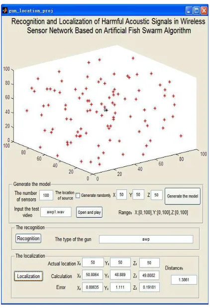
[image:4.612.89.294.458.549.2]We first generate the sensor network structure where the nodes are arranged with the artificial fish-swarm algorithm and harmful acoustic sources. The harmful source can be generated randomly or be a manual number in the given range. Then we input the file name of testing audio, and click “open and play” to determine the sound source. Next, in order to recognize the source of sound, we get the characteristic parameters from the sound in the process of LPC and compare the parameters with the subsistent ones in data base. After that, the name of the testing audio whose parameters are most similar to the subsistent parameters will be obtained. Finally, the system locates and shows the source of harmful acoustic signals. At the same time, the error can be obtained through the comparison between the value of calculation and the given location of the harmful source. The simulation results are shown in Fig. 5.
Figure 5The Simulation Of Whole System
5. RESULT AND ANALYSIS
[image:4.612.92.296.605.703.2]5.1 Optimized Sensor Network
We assume that the initial average coverage of the sensor network is 89.6%. It can reach around 96% after optimization with the artificial fish-swarm algorithm. We can conclude that the artificial fish-swarm algorithm optimizes the sensor network very well in that it not only reduces the redundancy of the nodes concentration but also improves the utilization efficiency of nodes.
5.2 Sound Recognition Based On LPC
To simulate, we choose gunshot as the harmful acoustic signal and set 10 shots as the standard audio. Then use 17 test audio which includes original audio and audio with noise to do the test. The accuracy rate is 94.1%, which is indeed a high recognition rate.
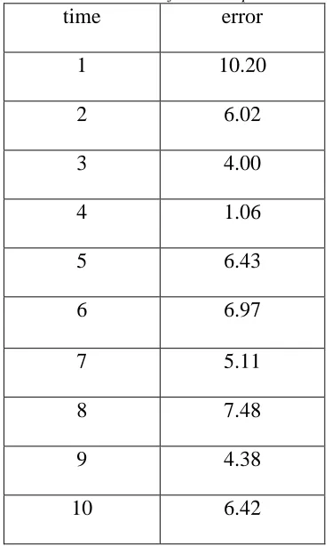
[image:5.612.101.288.339.646.2]5.3 Localization Of Harmful Acoustic Signals The errors of the 10 experiments are shown in table1:
Table 1: The Errors Of The 10 Experiments
We can calculate the average error is 5.8 which means that the harmful acoustic signals can be localized accurately.
6. CONCLUSIONS
In this paper, we have proposed a scheme for harmful acoustic signals recognition and localization based on artificial fish swarm algorithm
for wireless sensor network. We simulated the whole process including optimization of the sensor network, the recognition and location of harmful acoustic signals. We compared our system with the existing systems which realize the two aspects, separately. Simulation results confirm that the proposed system is of higher efficiency and better performance.
ACKNOWLEDGMENT
This work was supported in part by the research grant from National Natural Science Foundation of China (No. 61071122, No. 61271229), the Natural Science Foundation of Shandong Province (No. ZR2011FZ006), the New Century Excellent Talents from the Ministry of Education of China(NCET-11-0316) and the Independent Innovation Foundation of Shandong University.
REFRENCES:
[1] X.L. Li, Z.J. Shao and J.X. Qian, “An Optimizing Method Based on Autonomous Animats: Fish-swarm Algorithm”, Systems Engineering-Theory & Practice, Vol.22, No.11, November 2002, pp. 32-38.
[2] N. Li, C.R. Wang and C.L. Zhou, “Optimization Algorithm for Route Selection in Computer Networks Based on Artificial Fish-Swarm Algorithm”, Computer Science, Vol.32, No.8, 2005, pp. 218-220.
[3] J.W. Ma, G.L. Zhang and H. Xie, “Optimization of Feed-Forward Neural Networks based on Artificial Fish-Swarm Algorithm”, Computer Applications, Vol.24, No.10, Oct 2004, pp. 21-23.
[4] Y.J. Liu, “Artificial Fish Swarm Algorithm and Its Application in Coverage Optimization of WSN”.
[5] J.H. Duan, “Algorithm Research About Identification and Localization of Dangerous Acoustic Signals”.
[6] Z.C. Wang, “Optimization of Complex System Reliability Based on Artificial Fish-Swarm Algorithm”, Journal of Tai Zhou University, Vol.30, No.3, Jun 2008, pp. 28-31.
[7] MAKHOUL.J, “Linear prediction: A tutorial review”, Proc IEEE, Vol.63, 1975, pp. 561-580. [8] L.H. Zhang, B.Y. Zheng and Z. Yang, “A Study of Feature Parameters Based on LPC Analysis with Applications to Speaker Identification”, Journal of Nanjing University of Posts and Telecommunications, Vol.25, No.6, December 2005, pp. 1-6.
[9] Y.T. Chan, K.C. Ho, “A simple and efficient estimation for Hyperbolic Location”, IEEE
time
error
1
10.20
2
6.02
3
4.00
4
1.06
5
6.43
6
6.97
7
5.11
8
7.48
9
4.38
Trans Signal Processing, Vol.42, No.8, pp. 1905-1915.
[10] J.W. Zhang, B. Tang and F. Qin, “Application of Chan Location Algorithm in 3-Dimensional Space Location”, Computer Simulation, Vol.26, No.1, January 2009, pp. 323-326.
[11] C.F. Huang, Z.J. Shao and J.X. Qian, “The coverage problem in wireless sensor network”, Proc of ACM International Workshop on Wireless Sensor Networks and Applications, 2005, pp. 519-528.
[12] N. Xia, C.S. Wang and R. Zheng, “Sensor Redeployment Algorithm Based on Combined Virtual Forces in Three Dimensional Space”, ACTA AUTOMATICA SINICA, Vol.37, No.6, February 2012, pp. 295-302.
[13] H. Liu, Z.J. Chai and J.Z. DU, “Fish Swarm Inspired Underwater Sensor Deployment”, ACTA AUTOMATICA SINICA, Vol.38, No.2, June 2011, pp. 713-723.
[14] J. Jiang, L. Fang and H.Y. Zhang, “An Algorithm for Minimal Connected Cover Set Problem in Wireless Sensor Networks”, Journal of software, Vol.17, No.2, February 2006, pp. 175-184.
[15] Z.B. Zhang, S.S. Liu and G. Xu, “Vehicle Distance Measurement Based on Binocular Stereo Vision”, Journal of Theoretical and Applied Information Technology, Vol.44, No.2, 2012, pp. 179-184.
[16] P. Khuntia, P.K. Pattnaik, “Target Coverage Management Protocol for Wireless Sensor Network”, Journal of Theoretical and Applied Information Technology, Vol.35, No.1, 2012, pp. 20-25.
[17] A.A. Dhelaan, “Pyramid Based Data Gathering Scheme for Wireless Sensor Networks”, Journal of Theoretical and Applied Information Technology, Vol.29, No.2, 2011, pp. 92-99. [18] L.F. Xue, M.Y. Jiang and D.F. Yuan,
“Cloud computing model in web data mining”, Journal of Convergence Information Technology, Vol.7, No.22, 2012, pp. 585-592. [19] J. Tang, S.S. Liu and Z.M. Gu, “Prefetching in
Mobile Embedded System Can be Energy Efficient”, IEEE Computer Architecture Letters, Vol.10, No.1, 2011, pp. 8-11.
[20] L.G. Wang, Y. Hong and F.Q. Zhao, “Improved Artificial Fish Swarm Algorithm”, Computer Engineering, Vol.34, No.19, 2008, pp. 192-194.