HYBRID APPROACH FOR ENERGY OPTIMIZATION IN
CLUSTER BASED WSN USING ENERGY BALANCING
CLUSTERING PROTOCOL
1
T.SHANKAR, 2Dr.S.SHANMUGAVEL
1
Research Scholar, Department of ECE, Anna University, Chennai. India
2
Professor, Department of ECE, Anna University, Chennai. India
E-mail: 1
[email protected]
ABSTRACT
In recent times, the technology of wireless sensor network has a great impact on technical fields like wireless communication, information technology, electrical etc. However the major problem faced in this technology is that the sensor nodes run out of energy very quickly. Many routing protocols have been proposed to solve this problem mainly focussing on the accomplishment of minimizing the energy consumption in the sensor system. In this paper, two hierarchical protocols cluster based and chain based protocol for WSNs have been discussed. In both type of protocols some special nodes called cluster heads/chain heads acts as leader for a group of nodes. Each head collects data from its member nodes and forward it to the sink (base station). Here consider a homogeneous network where all the nodes in the network have uniform and limited resource energy. So it is essential to avoid quick depletion of head nodes. Hence every node in the network takes their turn to act as head but only for a limited period of time. Energy saving in these approaches can be obtained by cluster formation, head election and data aggregation at the head nodes. The proposed Energy Balancing Clustering Protocol (EBCP) which uses Bacterial Foraging Optimization Algorithm in electing the cluster head. The simulation results shows that the proposed protocol extends the life time of the network when compared with Energy Efficient Unequal Clustering (EEUC)and PEGASIS with Double Cluster Head technique(PDCH).
Keywords: BFO, Cluster Head, PEGASIS, Static clustering, WSN
1. INTRODUCTION
Wireless Sensor Networks(WSN) have gained world-wide attention in recent years due to the advances made in wireless communication, information technologies and electronics field [1],[2],[3].The concept of wireless sensor networks is based on a simple equation: Sensing + CPU + Radio = Thousands of potential applications [4],[5][6]. It is a natural sensing technology where tiny, autonomous and compact devices called sensor nodes or motes deployed in a remote area to detect phenomena, collect and process data and transmit sensed information to users. The development of low-cost, low-power, a multifunctional sensor has received increasing attention from various industries. Sensor nodes or motes in WSNs are small sized and are capable of sensing, gathering and processing data while communicating with other connected nodes in the network, via radio frequency (RF) channel. At
heads in every round[9]. So the nodes’ die rate will decrease and eventually it will increase network life time. The remaining part of the paper is organized as follows: we discuss the network, radio models and related work , is briefly discussed in Section 2. In Section 3 we discuss the Energy Efficient protocols in WSN Section 4 describes implementation of the protocols. In Section 5, we simulate the proposed protocol by using MATLAB simulator and compare its performance with other prevalent routing protocols. Finally, some conclusions are drawn in Section 6. This paper describes the two different protocols, energy efficient unequal clustering (EEUC) protocol and pegasis with double cluster head (PDCH) protocol followed by a bio inspired algorithm namely bacterial foraging optimization algorithm (BFOA). These three protocols will follow different cluster head selection technique and different transmission technique.
2. RELATED WORK
In 1981, Baker and Ephremides proposed a clustering algorithms called ―Linked cluster algorithm (LCA) [10] for wireless networks. To enhance network manageability, channel efficiency and energy economy of MANETS, Clustering algorithms have been investigated in the past. Lin and Gerla investigated effective techniques to support multimedia applications in the general multi-hop mobile ad-hoc networks using CDMA based medium arbitration in [11]. Random competition based clustering (RCC) [12] is applicable both to mobile ad hoc networks and WSN. RCC mainly focuses at cluster stability in order to support mobile nodes. Some of well known clustering algorithms for mobile ad hoc networks presented in the literature are Cluster Gateway Switch Routing Protocol (CGSR) [13], Cluster-Based Routing Protocol (CBRP) [14], Weighted Clustering Algorithm (WCA) [15]. A survey of clustering algorithms for mobile ad hoc networks has been discussed in [16]. In recent years, insect sensory systems have been inspirational to new communications and computing models like bio inspired routing Biological synchronization phenomena have great potential to enable distributed and scalable synchronization algorithms for WSN.
THE ROUTING PROTOCOLS FOR NETWORK STRUCTURE
Flat based routing
In these protocols, all nodes have assigned equal roles in the network. The well known protocols considered in flat based routing are:
• Sequential Assignment Routing (SAR),
• Directed Diffusion,
• Energy Aware Routing (EAR) etc.
Sequential Assignment Routing proposed was one of the first protocols for WSN that considered QoS issues for routing decisions. The objective of SAR algorithm is to minimize the average weighted QoS metric throughout the lifetime of the network .SAR makes a routing decision based on three factors: energy resources, QoS planned for each path, and the packet‘s traffic type, which is implemented by a priority mechanism. To resolve reliability problems, SAR uses two systems consisting of a multipath approach and localized path restoration done by communicating with neighboring nodes.
Directed diffusion (DD) [21] is a data-centric and application aware paradigm since all data generated by sensor nodes are named by attribute value pairs. The objective of the directed diffusion paradigm is to aggregate the data coming from different sources by deleting redundancy, which drastically reduces the number of transmissions. Energy Aware Routing [22] is a reactive protocol to increase the lifetime of the network.
Hierarchical based routing
It is also known as cluster-based routing. In these protocols, the nodes can play different roles in the network and normally the protocol includes the creation of clusters. Additionally, designations of tasks for the sensor nodes with different characteristics are also performed.
LEACH
CH nodes as routers to the base-station. All the data processing such as data fusion and aggregation are local to the cluster. LEACH forms clusters by using a distributed algorithm, where nodes make autonomous decisions without any centralized control.
PEGASIS
Power-Efficient Gathering in Sensor Information Systems (PEGASIS) [27] protocol is a LEACH-inspired protocol. PEGASIS is not exactly a cluster-based protocol, as nodes are not explicitly grouped into clusters. PEGASIS is instead a chain based approach, in which each node only communicates with a close neighbour and takes turns to transmit to the BS, thus reducing the amount of energy spent per round. This approach distributes the energy load evenly among the sensor nodes in the network. The PEGASIS protocol is designed for a WSN containing homogeneous and energy-constrained nodes, with no mobility. The BS (sink) is fixed and far away from nodes. The radio model adopted is the first-order radio model, same as the LEACH protocol. Using this model, energy efficiency can be improved by minimizing the amount of direct transmissions to the sink node. This idea is common to the LEACH protocol, in which clustering is used to reduce both the duty cycle of the nodes and direct transmissions to the BS.
HEED protocol is a distributed single-hop clustering routing protocol for Wireless Sensor Networks, in which selecting CHs based on both residual energy of each node and communication cost. It has the advantages in increasing the network lifetime and having a constant algorithm complexity
Bio-inspired routing
In recent years insect sensory systems have been inspirational to new communications and computing paradigms, which have lead to significant advances like bio inspired routing [26]. The most popular ACO (Ant Colony Optimization) is a colony of artificial ants is used to construct solutions guided by the pheromone trails and heuristic information they are not strong or very intelligent; but they successfully make the colony a highly organized society. Swarms are useful in many optimization problems. A swarm of agents is used in a stochastic algorithm to obtain near optimum solutions to complex, non-linear optimization problems [27]. Swarm Intelligence
Optimization Based Routing Algorithm [28] works
with the objective to balance global energy
consumption and avoiding some node‘s premature energy exhausting..
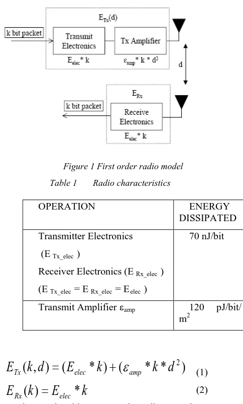
First Order Radio Model
Currently, there is a great deal of research in the area of low-energy radios. Different assumptions about the radio characteristics, including energy dissipation in the transmit and receive modes, will change the advantages of different protocols. In this work, simple radio model is taken where the radio dissipates Eelec = 70 nJ/bit to run the transmitter or
receiver circuitry and E amp = 120 pJ/bit/m2 for the
transmit amplifier to achieve an acceptable Eb / No
(see Figure 1 and Table 1). These parameters are slightly better than the current state-of-the-art in radio design. Assume an r2 energy loss due to channel transmission. Thus, to transmit a k-bit message a distance d using the radio model, the radio expands:
[image:3.612.313.555.318.719.2]Figure 1 First order radio model
Table 1 Radio characteristics
(1)
(2)
and to receive this message, the radio expends:
OPERATION ENERGY
DISSIPATED
Transmitter Electronics
(E Tx_elec )
Receiver Electronics (E Rx_elec )
(E Tx_elec = E Rx_elec = Eelec )
70 nJ/bit
Transmit Amplifier εamp 120 pJ/bit/
m2
k
E
k
E
d
k
k
E
d
k
E
elec Rx
amp elec
Tx
*
)
(
)
*
*
(
)
*
(
)
,
(
2=
+
E Rx (k) = ERx_elec(k) (3)
E Rx (k) = Eelec* k (4)
For these parameter values, receiving a message is not a low cost operation; the protocols should thus try to minimize not only the transmit distances but also the number of transmit and receive operations for each message. Assumption is made that the radio channel is symmetric such that the energy required to transmit a message from node A to node B is the same as the energy required transmitting a message from node B to node A for a given SNR.
3. ENERGY EFFICIENCT PROTOCOLS IN WSN
Initially when the sensor system was introduced direct transmission from node to the destination was used. But in this transmission mode the energy consumption of the nodes which are far from the BS will be high. This is because the first order radio model shows that energy required to transmit Etxer
is directly proportional to the square of the distance (d). And this type of nodes will die very quickly. So to reduce the transmission energy, transmission distance is to be reduced. For this purpose this paper discusses two types of hierarchy protocols. They are:
• Cluster based protocol
• Chain based protocol
CLUSTER BASED PROTOCOL
In this type of protocols entire network is divided into small areas as shown in the Figure 2 called clusters. And BS informs each node to which cluster they belong. After assigning all nodes into clusters BS will elect a node from each cluster as head (cluster head-CH) and informs the other nodes in the cluster. During the transmission phase nodes will transmit the data to the respective cluster head. Due to this type of transmission the distance to which the data is to be transmitted is reduced. The function of the cluster head is to gather the data from its cluster nodes and fuse it. After fusing the data, this fused data has to be sent to the base station. Thus BS receives data only from CHs, so the number of reception at the BS also reduced. All these modifications in the network show that the energy consumption by the nodes is reduced.
Figure2 Clustering Technique
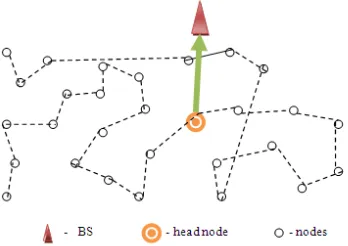
[image:4.612.329.503.496.619.2]CHAIN BASED PROTOCOL
Figure 3 shows how the chain transmission is performed in the network. Initially the transmission starts from the farthest node from the BS. This node will transmit its data to its nearest neighbour. The node which receives the data will aggregate the received data with its own data and then transmits the aggregated data to its nearest neighbour node. This process continues till the data in the network reaches the node (head) which transmits the aggregated data to the BS. In this, each node will take its turn in transmitting the data to BS. As the node communicates with only to its nearest neighbour the distance of communication is much reduced and also the head node will have maximum of two receptions. Due to this lot of energy is saved.
Figure 3 Chain Based Network
EEUC - ENERGY EFFICIENT UNEQUAL CLUSTERING
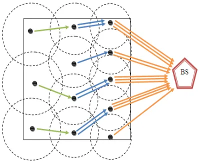
The main objective of this protocol is trying to wisely design the network with clustering and multi hop routing scheme to extend the network lifetime. This protocol adopts both the rotation of cluster heads and choosing cluster heads with more residual energy. Furthermore, it introduces an unequal clustering mechanism which is an effective method to deal with the hot spots problem. It can prevent the premature creation of energy holes in wireless sensor networks. Figure 4, gives an overview of the EEUC mechanism, where the circles of unequal size represent the clusters of unequal size and the traffic among cluster heads illustrates the multi hop forwarding method. It shows that the node’s competition range decreases as its distance to the base station decreasing. The result is that clusters closer to the base station are expected to have smaller cluster sizes, thus they will consume lower energy during the intra-cluster data processing, and can preserve some more energy for the inter-cluster relay traffic.
[image:5.612.90.289.382.543.2]
Figure 4 Unequal Clustering Mechanism
The cluster heads closer to the base station act as
routers of heads farther away from the base station during delivering data to the base station. The reason is that multi hop communication is more realistic because nodes may not be able to communicate directly with the base station due to the limited transmission range.
Cluster Head Selection
In EEUC, cluster heads are selected based on a competitive algorithm where the selection is primarily based on residual energy of each node.
First, several tentative cluster heads are selected to compete for final cluster heads. Every node can become a tentative cluster with the probability T, a predefined threshold. Each head calculates the competition radius in which the energies are to be compared with those of tentative CHs, the one with maximum energy is elected as new CH. In the case of tie in energies, the node with smaller node ID is chosen as CH. The energy consumed in intra-cluster processing varies proportionally to the number of nodes within the cluster. The cluster heads closer to the base station should support smaller cluster sizes because of higher energy consumption during the inter-cluster multi hop technique. Thus more clusters should be produced nearer to the base station. The competition range of the CH is given by
𝑠𝑖.𝑅𝑐𝑜𝑚𝑝=�1− 𝑐𝑑𝑑𝑚𝑎𝑥−𝑑(𝑠𝑖,𝐵𝑆)
𝑚𝑎𝑥−𝑑𝑚𝑖𝑛 � 𝑅𝑜
(5) where 𝑠𝑖 is the current CH over which radius of
competition (𝑅𝑐𝑜𝑚𝑝 is calculated. 𝑑𝑚𝑎𝑥and 𝑑𝑚𝑖𝑛 are the maximum and minimum distance between sensor nodes and BS, .𝑑(𝑠𝑖, 𝐵𝑆) denotes the distance between current CH and BS. c is a constant between 0 and 1.Ro is the maximum completion radius which is pre-defined. After the cluster heads have been selected, each node joins its closest CH thereby forming the clusters.
INTER-CLUSTER MULTI HOP ROUTING
When cluster heads delivers their data to the base station, each CH first aggregates the data from its cluster members, and then sends the packet to the base station via multi hop communication. If a node’s distance to the base station is smaller than TDMAX (a predefined threshold), it transmits its data to the base station directly, and else it should find a relay node which can forward its data to the base station. Relay node can be chosen based on two parameters residual energy and link cost, a trade off should be made between these two.
In this protocol, relay node is the one with more residual energy from two smallest link costs. The link costs are calculated as
𝑑2
𝑟𝑒𝑙𝑎𝑦= 𝑑2�𝑠𝑖,𝑠𝑗�+𝑑2(𝑠𝑖,𝐵𝑆) (6)
Where 𝑠𝑗 is the current CH and 𝑠𝑖 is the relay node, it will send its own data together with forwarding data directly to base station.
The PEGASIS is a chain based hierarchical protocol. In chain based transmission generally energy consumption is very less compared to cluster based or direct transmissions. But Data transmission will create time-delay because the probability of long chain is always high. Also the method of choosing cluster head is not suitable for load balancing. To overcome these problems a protocol with the combination of both clusters and chains were introduced. Along with this double cluster head technique is also used in this protocol. The following section will take you to in depth of the PDCH protocol.
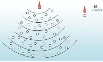
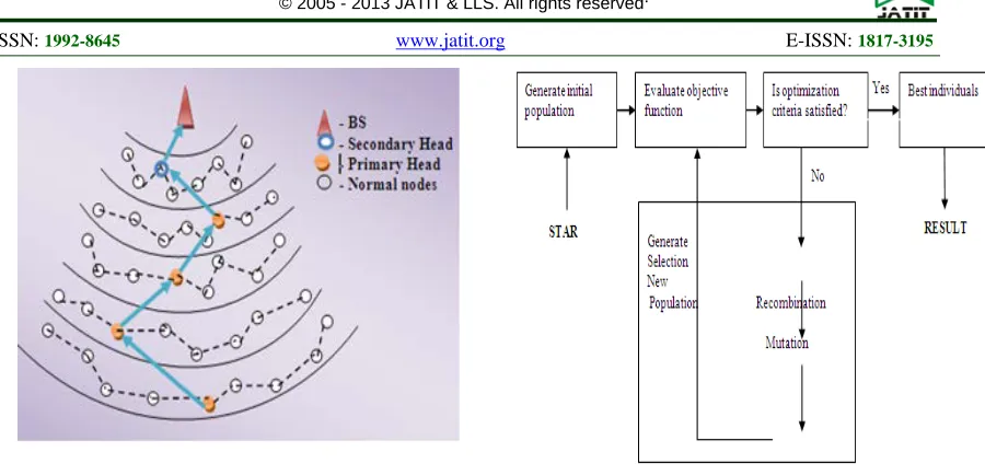
[image:6.612.103.279.454.561.2]In the network structure, base station (BS) is assumed to be at the centre of a circle. With reference to the centre (BS) the network is divided into levels. Every node's distance to BS decided the level which it belongs to. The BS will pre- configure the number of levels. Every Node receives a signal from the BS, and then according to the signal strength the distance to the node from BS is detected. The number of nodes and the density of distribution, the location of BS and so on will affect the number of level in the network. Every level has ID. The first level has 0 as its ID, it belong to BS. The second level has 1, nodes belong to this level is the most closest to BS and so forth. Look at the Figure 5, there have 5 levels.
Figure 5 Clustering Hierarchy
Notice that this hierarchy always run at the start, and once success, it will not be change in the whole process. This can save energy compare to frequently stratify in every round. Then the chain is build in every level, the nodes belong to different levels can't build in the same chain, only the nodes with same ID can be built in the same chain. Chain formed among the cluster nodes is called branch chain and head selected in that chain is called primary head. Chain formed among the primary heads is called main chain and the head in the main chain is called secondary head.
CLUSTER HEAD SELECTION Selection of primary head
The selection of primary head will base on the residual energy of the nodes. In homogenous networks, initially all the nodes are provided with equal amount of energy. During the first round of transmission primary head will be randomly selected within the respective cluster nodes. After the first round of transmission, every node consumes some energy which is not equal for every node. Therefore, after first round of all the nodes in the cluster, the node which has maximum residual energy will be selected as a head. In case if there are multiple nodes with same maximum energy then the node with least id will be selected as head.
Selection of secondary head
The primary heads in the network one primary head will act as a secondary head.Theselection of secondary head will base on the distance of primary head from the base station. The primary head which is nearer to the base station will be selected as a secondary head. But in the above mentioned network structure, the head which is nearer to the BS is always the head from level 1. Therefore the primary head from level 1 will be acting as a secondary head throughout the network life time.
FUNCTION OF EACH HEAD Primary head
The main function of the primary head is to collect the data from all the nodes in the cluster and aggregate that data. Data aggregation means head will check for the redundant information, and removes it. After aggregating all the data, primary head will transmit this data to secondary head through same chain transmission.
Secondary head
Figure 6 Transmission Mechanism In PDCH
Figure 6 shows how the transmission is done in the network using double cluster head technique. As discussed primary CH will collect all the data in the cluster and transmits the data to secondary CH through the nearest primary heads.
BACTERIAL FORAGING OPTIMIZATION
Bacterial Foraging Optimization (BFO) is an Evolutionary based algorithm. Evolutionary algorithm is stochastic search methods that mimic the metaphor of natural biological evolution. Evolutionary algorithms operate on a population of potential solutions applying the principle of survival of the fittest to produce better and better approximations to a solution. At each generation, a new set of approximations is created by the process of selecting individuals according to their level of fitness in the problem domain and breeding them together using operators borrowed from natural genetics. This process leads to the evolution of populations of individuals that are better suited to their environment than the individuals that they were created from, just as in natural adaptation.
PRINCIPLE OF EVOLUTIONARY ALGORITHMS
[image:7.612.94.544.63.280.2]Evolutionary algorithms model natural processes, such as selection, recombination, mutation, migration, locality and neighbourhood. Figure 7 shows the structure of a simple evolutionary algorithm.
Figure 7 Structure Of A Single Population Evolutionary Algorithm
From the above discussion, it can be seen that evolutionary algorithms differ substantially from more traditional search and optimization methods. The most significant differences are eevolutionary algorithms search a population of points in parallel, not just a single point. These algorithms do not require derivative information or other auxiliary knowledge; only the objective function and corresponding fitness levels influence the directions of search. Evolutionary algorithms use probabilistic transition rules, not deterministic ones.
BACTERIAL FORAGING OPTIMIZATION FOR CLUSTER HEAD SELECTION
Bacterial Foraging Optimization (BFO) is a population-based numerical optimization algorithm. In recent years, bacterial foraging behavior has provided rich source of solution in many engineering applications and computational model. It has been applied for solving practical engineering problems like optimal control, harmonic estimation, channel equalization etc. In this paper, BFO has been used for cluster head selection to provide improved energy efficiency in routing. This section discusses process of cluster head selection using BFO algorithm. The process of cluster head selection involves application of a clustering algorithm.
BACTERIAL FORAGING ALGORITHM
optimization problems. E. coli is a common type of bacteria. An E. coli bacterium alternates between running and tumbling. If it swims up nutrient gradient the E. coli will swim longer. If it swims down nutrient gradient the E. coli will search again to avoid unfavourable environments. Events can occur such that all the bacteria in a region are killed or a group is dispersed into a new part of the environment. Elimination and dispersal events have the effect of possibly destroying chemotactic progress, but they also have the effect of assisting to place bacteria near good food sources. When the bacteria are moving, they can release the attractant aspartate to congregate into groups and move as concentric patterns of groups with high bacterial density. If the basic goal is to find the minimum of
J(θ), θ∈RP (7) θ is the position of a bacterium, and J(θ) represents an attractant-repellant profile (J < 0, J = 0, and J > 0 represent the presence of nutrients, a neutral medium, and the presence of noxious substances, respectively).
P (j, k, l) = {θi (j, k, l) / i =1, 2,…S } (8)
represents the positions of each member in the population of the S bacteria at the jth chemo tactic step, kth reproduction step, and lth elimination-dispersal event. J (i, j, l) denotes the cost at the location of the ith bacterium θi (j, k, l) ∈RP. Nc is
the length of the lifetime of the bacteria as measured by the number of chemo tactic steps. The tumble step can be represented as follows
θi
(j +1, k, l) = θi(j, k, l) + C(i)φ(j) (9) φ(j) is generated as a unit length random direction. C(i) >0 is the size of the step taken in the random direction specified by the tumble. Another chemo tactic step of size C(i) in this same direction will be taken if the cost J(i, j+1, k, l) at θi(j+1, k, l) is better than at θi
(j, k, l). Ns is the maximum
number of chemo tactic steps.
The function Jicc (θ) is used to model the
cell-to-cell swarming step.
𝐽𝑐𝑐(𝜃) =∑ 𝐽𝑠𝑖=1 𝑐𝑐𝑖 (10)
= �[
𝑠
𝑖=1
− 𝑑𝑎𝑡𝑡𝑟𝑎𝑐𝑡exp (−𝑤𝑎𝑡𝑡𝑟𝑎𝑐𝑡��𝜃𝑗− 𝜃𝑗𝑖�2) 𝑝
𝑗=1
]
+�[
𝑠
𝑖=1
− ℎ𝑟𝑒𝑝𝑒𝑙𝑙𝑎𝑛𝑡exp (−𝑤𝑟𝑒𝑝𝑒𝑙𝑙𝑎𝑛𝑡��𝜃𝑗 𝑝
𝑗=1
− 𝜃𝑗𝑖�2)]
(11)
where dattract is the depth of the attractant
released by the cell. Wattract is a measure of the
width of the attractant signal. hrepellant =dattract, which
is the height of the repellant effect. wrepellant is a
measure of the width of the repellant. θ = [ θ1,….
θp]T is a point on the optimization domain, which
can have P dimension.
The goal is to find the minimization of
J (i, j, k, l) + Jcc (θi(j, k, l)). (12)
The bacteria will try to find nutrients, avoid noxious substances, and at the same time try to move toward other bacteria, but not too close to them. The Jcc(θi (j, k, l)) function dynamically
deforms the search landscape to represent the desire to swarm. After Nc chemo tactic steps, a
reproduction step is taken. Nre is the number of
reproduction steps. In the reproduction steps healthiest bacteria split, the same number of unhealthy ones are killed. Ned is the number of elimination-dispersal steps with probability ped.
EBCP-ENERGY BALANCING CLUSTERING PROTOCOL
Energy Balancing Clustering protocol aims at balancing the energy among the nodes in every cluster and reducing the energy dissipation of the cluster-heads. This protocol is briefly discussed in three phases. They are cluster formation phase, cluster head selection phase, steady phase.
Cluster formation phase
While forming clusters, initially tentative head nodes called auxiliary cluster heads are selected. The node which is far from the BS is selected as first auxiliary head. This auxiliary head will select the nearest fixed number of nodes as its members. After the formation of first cluster, the farthest node among the un-clustered nodes will be selected as the second auxiliary cluster head and this process continues till the entire nodes in the network are clustered. The network owns the same auxiliary cluster-heads and every auxiliary cluster-head owns the same members. But the auxiliary cluster-heads are not the final cluster-heads, and BFOA algorithm is used in order to find the main cluster heads.
Cluster head selection phase
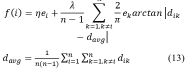
cluster heads in electing the main cluster head. As discussed earlier in the process of foraging, bacteria will undergo swim and tumble before reaching the most nutrient position. A fitness function is used for balancing energy consumption in each cluster. By using this, the position in the cluster from where the energy can be balanced is found. Balancing means the nodes which are closer to the position can have less energy and the node which is far should have highest energy. The fitness function, f (i) is given below
𝑓(𝑖) =𝜂𝑒𝑖+𝑛 −𝜆 1 � 2𝜋 𝑒𝑘𝑎𝑟𝑐𝑡𝑎𝑛 𝑛
𝑘=1,𝑘≠𝑖
�𝑑𝑖𝑘
− 𝑑𝑎𝑣𝑔�
𝑑𝑎𝑣𝑔=𝑛(𝑛−11 )∑ ∑𝑛𝑖=1 𝑛𝑘=1,𝑘≠𝑖𝑑𝑖𝑘 (13)
Where i is the current node for which fitness is to
be computed, 𝑒𝑖 is the energy of the ith node, k indicates the other nodes in the cluster(except i),𝑑𝑖𝑘is the distance between ith and kth nodes. 𝑑𝑎𝑣𝑔 is the average distance within cluster, n is the no. of nodes in the cluster.This fitness function is similar to the health function in BFOA. The node that has maximum fitness value will be elected as main cluster head. This function takes the residual energy and positions of nodes into consideration. It tries to balance the energy consumption in the cluster.
𝐽(𝑖) =𝑓(𝑖) (14)
Now, the problem of finding the final cluster-head can be transformed into solving a maximum value problem. Solving the equation for maximum value will result in a most suitable position of the cluster head in each cluster. But it is not necessary that position should have node. Then this most suitable position is mapped into one of the real positions of the nodes in the cluster. The node in this corresponding position will be selected to be the final cluster-head. And that is found using the following equation.
𝑑𝑚𝑖𝑛=𝑚𝑖𝑛{‖𝑃𝑏− 𝑃1‖,‖𝑃𝑏− 𝑃2‖… . .‖𝑃𝑏
− 𝑃𝑖‖… . .‖𝑃𝑏− 𝑃𝑛‖}
(15)
Where Pb is the most suitable position of cluster head found using BFO algorithm,Pi is the position of ith the nodes in the cluster. N is the no. of nodes in the cluster.
The real position of a certain node with 𝑑𝑚𝑖𝑛 will be chosen to be the position of the final
cluster-head, which means that the nearest node from the Pb in the cluster will act as the final cluster-head.
Steady phase
This phase generally discuss about the communication part in the network. That is how the data from nodes to CH and CH to BS is transmitted. This protocol uses direct transmission within the cluster. In this type of transmission the nodes in every cluster will transmit their sensed data directly to the respective cluster heads.CH will allocate each node with a time slot. And when the node time comes it will transmit and rest of the time it will be in sleep mode. Cluster heads aggregates the data and transfers it to the base station.
4. IMPLEMENTATION OF THE PROTOCOLS USING MATLAB
The detailed explanation of the EEUC, PDCH, EBCP protocols is given in the previous chapter. In this chapter the constraints that are considered in designing the network are discussed and the algorithm steps which are used in implementing those protocols and flow charts of the protocols. It is also going to discuss the advantages and disadvantages if any of these protocols and propose the modifications done in overcome those disadvantages.
NETWORK DESIGN
[image:9.612.102.287.230.304.2]Table2 shows the required parameters whose initial values are assumed as follows
Table 2 Parameters and their initial values
Parameter Value
Sensor field region 200*200
Base station location (100,250)
No. of nodes 300
Initial energy 0.5J
Data Packet length 4096bits
1 Round 0.2 sec
EEUC IMPLEMENTATION
STEP 1
Initially network is created using ‘rand’ command using the above initial parameters. Base station is plotted at the given location.
The entire sensor network is divided into regions based on the distances from the BS. Initially some random nodes are assigned as cluster heads for clustering purpose. The probability of number of nodes to become initial cluster heads is higher in the region nearer to BS than other regions. This is because each cluster head corresponds to a cluster thereby forming more number of clusters of smaller sizes nearer to the base station.
STEP 3
After selecting the initial cluster heads, all the nodes in the respective regions computes distances to all cluster heads and each node joins the corresponding cluster head of the same region which is of minimum distance to it. Proceeding in this manner, the entire network is divided into clusters.
STEP 4
After forming the clusters, energy dissipation in case of intra cluster communication is calculated i.e., for data transmission and reception, first order radio model is used as discussed in the chapter 2.
STEP 5
After forming the clusters, new CHs are elected after every round. From the remaining nodes, other than CHs, tentative cluster heads are chosen based on pre-defined threshold value. For each cluster head a competition radius is calculated and the energies of tentative CHs are compared with the current CH. The node having maximum energy among these is elected as the new CH. Each CH first aggregates the data from its cluster members, and then sends the packet to the base station via multi hop communication. If a node’s distance to the base station is smaller than TDMAX (a predefined threshold), it transmits its data to the base station directly, and otherwise it should find a relay node in the next level which can forward its data to the base station. Relay node is found using the Euclidean distance formula as discussed in above chapter and the data transmission part is similar to that in the step 4.
Now this completes one round of transmission. STEPS 4 to 6 are repeated for several rounds of transmission. Check for the dead nodes after completion of each round. Dead nodes are the nodes with residual energy less than or equal to zero. If dead nodes are found then the node is removed from the corresponding cluster. And number of nodes that are dead in each round are counted and saved in an array. The value of sum of residual energies of all alive nodes is found in every
round and saved in another array. Now the plot is made for the number of alive nodes in each round and residual energy of the network in each round.
MODIFIED EEUC (M-EEUC)
we consider base station (BS) to be far away from the network. But the result of this protocol can be further improved by considering the change in base station metrics and by changing the network topology.
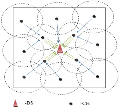
[image:10.612.332.522.355.526.2]As shown in the figure 8, the BS is placed at the centre of the network region. This helps in changing the network topology. The cluster heads closer to the BS have smaller cluster sizes to preserve some energy for the inter-cluster data forwarding, which can balance the energy consumption among cluster heads and prolong the network lifetime. We can observe that the transmission from any CH node to the BS is now reduced to single-hop distance.
Figure 8 Improved Unequal ClusteringMechanism
In this improvement, the distance parameter is enhanced, because the transmission distances from various cluster heads to BS is reduced. And also the network topology is changed accordingly, placing the smaller clusters around the base station eliminating the hot spot problems in multi-hop routing paths.
PDCH IMPLEMENTATION
STEP 1
Initially network is created using ‘rand’ command using the above initial parameters. Base station is plotted at the given location.
Now the distance from base station to all other node in the network is found using Euclidean distance formula.
𝑑𝑖=�(𝑥𝑏𝑠− 𝑥𝑖)2+ (𝑦𝑏𝑠− 𝑦𝑖)2 (16)
Where
𝑑𝑖 is the 𝑖𝑡ℎnode distance from base station.
𝑥𝑏𝑠,𝑦𝑏𝑠 are the coordinates of the base station.
𝑥𝑖,𝑦𝑖 are the coordinates of the 𝑖𝑡ℎ node.
Now the levels are formed based on the distance from base station and each level is given an id. In this the nodes which are less than or equal to 100 meters comes under first cluster (level id=1). 100 to 150 come under second cluster (level id=2), 150 to 200 come under third cluster (level id=3) and 200 to 250 come under fourth cluster (level id=4).
STEP 3
After forming the clusters, head node is elected in each cluster. In this protocol the head node is elected based on the residual energy of the nodes. The node which has maximum residual energy will be elected as a cluster head. But in the initial case all the nodes will have same energy. So in the first round of transmission some random node is elected as cluster head.
CH= Node with maximum residual energy
STEP 4
After electing the cluster head, a chain is formed using the nodes in the cluster. Node with same level id can only involve in chain formation. And the flow chat used for the formation of chain is shown in the figure.
STEP 5
After forming the chains in each cluster data transmission is done in the cluster. For data transmission and reception, first order radio model which is discussed in the previous chapter is used. And the algorithm used in routing the data packet is given below.
STEP 6
Now the data available in the cluster nodes is transmitted to cluster head. These CHs are known to be primary heads. Now all the CHs are
considered to form a separate cluster. And of these nodes the node nearer to the base station is elected as head which is known as secondary cluster. And again a chain is formed among these nodes and data is transmitted to secondary head. This secondary head node will transmit that data to base station.
Now this completes one round of transmission. STEPS 3 to 6 are repeated for several rounds of transmission. Check for the dead nodes after completion of each round. Dead nodes are the nodes with residual energy less than or equal to zero. If dead nodes are found then the node is removed from the corresponding cluster. And number of nodes that are dead in each round are counted and saved in an array. The value of sum of residual energies of all alive nodes is found in every round and saved in another array. Now the plot is made for the number of alive nodes in each round and residual energy of the network in each round.
Advantages
Cluster head selection is based on the residual energy of the nodes. Transmission distance is very much reduced due to chain transmission. The function of single cluster head is divided between two. Clusters are fixed and no need for clustering every time.
MODIFIED PDCH (M-PDCH)
Modified PDCH
In the above discussed process of cluster head selection we consider only the residual energy of the nodes. But the result of this protocol can be still improved by considering the distance parameter. The equation for cluster head selection is given by
𝑟𝑎𝑡𝑖𝑜=𝐸𝑐𝑜𝑛
𝐸𝑟𝑒𝑠 (17)
𝐸𝑐𝑜𝑛 is energy consumed if the node is selected as
cluster head,
𝐸𝑟𝑒𝑠is the residual energy of the node
The node with least ratio is selected to be cluster head. For the ratio to be least the numerator energy consumed should be less and the denominator residual energy should be high. But the energy consumption will be less only when distance of transmission is less.
Therefore the equation shows that, the nearest node with maximum residual energy is selected as cluster head.
EBCP IMPLEMENTATION
Initially network is created using ‘rand’ command using the above initial parameters. Base station is plotted at the given location.
STEP 2
Now the distance from base station to all other node in the network is found using Euclidean distance formula.
𝑑𝑖=�(𝑥𝑏𝑠− 𝑥𝑖)2+ (𝑦𝑏𝑠− 𝑦𝑖)2 (18)
𝑑𝑖 is the 𝑖𝑡ℎnode distance from base station.
𝑥𝑏𝑠,𝑦𝑏𝑠 are the coordinates of the base station.
𝑥𝑖,𝑦𝑖 are the coordinates of the 𝑖𝑡ℎ node.
Now the farthest node from the base station is found and is taken as first auxiliary head. After finding the first auxiliary head, distances of all other nodes from the auxiliary head is found using the same Euclidean formula. After finding the distance chose the nearest fixed number of node as its members. After forming the first cluster, second auxiliary cluster head, the farthest node from the base station among the un-clustered nodes is selected and again its members are selected as discussed above. This process continues till all the nodes in the network are clustered.
STEP 3
In this the final cluster head is elected using bacterial foraging optimization algorithm. A function called fitness function is defined using BFO algorithm. The fitness function, f (i) is given below equation(13) is applied to every node in the cluster. The node which has maximum value of the fitness function is selected as main cluster head.
STEP 4
After electing the main cluster heads, the data packet is transmitted by all the nodes in the cluster to its main head directly. The main cluster head will gather all the data from the cluster and transmits it to base station. Now the CHs transmit the data to BS, it completes one round of transmission. In every round STEP 3 and STEP 4 are repeated to make sure that the energy in the cluster is balanced. After completion of each round the network is checked for the dead nodes and the residual energy of the network. The values of dead node and residual energy are stored in different array. Plot between alive nodes (total nodes-dead nodes), rounds and residual energy of the network, rounds are made.
Advantages
The main advantage in this protocol is the CH is elected in such a way that the energy in the network is balanced i.e., the node which is far from the CH will have highest energy and the node which is nearer will have lowest energy. Due to this the percent of energy spent by all the nodes in the cluster will be almost equal. So the nodes which are far can also live for the same time as the nearer will. Due to this life time of the network is extended.
CHAIN BASED EBCP (C-EBCP)
In the transmission phase of EBCP protocol direct transmission between nodes and the cluster head is used. But it is seen that the chain transmission is more effective than the direct transmission in extending the network life time. Therefore the protocol is rebuilt using the chain transmission within the cluster. In implementing the protocol, the implementation steps (step 1 to step 3) are same as discussed in the above session. In step 4 instead of going for direct transmission within the cluster, the data is transmitted through chain. In this, farthest node from the CH will start the transmission. It sends its data to the nearest neighbour node. That node will fuse the received data with its own data and then transmits it to its nearest node and the process continues till all the nodes data reached to CH.
5 SIMULATION AND RESULTS
SIMULATION METRICS
The main objective of the simulation study is to evaluate the performance of each protocol. Evaluation is made based on the following two metrics
• Number of nodes alive.
• Residual energy of the network.
Number of nodes alive
The performance of a network depends on the lifetime of its nodes. If the lifetime of the nodes is high then the network performs well and also transmits more data to the base station.
Residual energy of the network
The residual energy of the network with respect to number of rounds is analyzed .The greater the residual energy of the network, the better is the algorithm.
Figure 9 Initial Clustering In PDCH Protocol
Figure 10 Chain Formations In Each Cluster
Figure 9 shows how the nodes are deployed in the field region and how these nodes are divided into clusters. Each cluster is indicated with different colours. It also shows that the base station is located at (100,250) which is 50 meters away from the field region. Figure 10 shows the chain transmission in every cluster and also among the cluster heads. Finally the secondary cluster head which is square in shape and black in colour will transmit the entire data in the network to the base station.
Figure 11 Comparison Of Number Of Nodes Alive In The System Among PDCH&M-PDCH
[image:13.612.106.299.302.460.2]Figure 11 shows the comparison result of the number of nodes alive after every round in both PDCH and M-PDCH protocols. The round at which the nodes alive become zero is called the life time of the network in term of rounds. As per the figure the life time of the network in PDCH protocol is 2156 rounds where as in M-PDCH it is 2423 rounds.
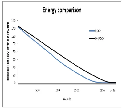
Figure 12 Residual Energy Of The Network In PDCH&M-PDCH
[image:13.612.324.522.398.575.2]EBCP&C-EBCP
Figure13 Cluster Formation In EBCH Protocol
Figure 13 shows how the clusters are formed in the EBCP protocol and each cluster is denoted with different colours. In each cluster the node denoted as red coloured square box will indicate the auxiliary cluster head and node denoted with black coloured star will indicate the main cluster head that is elected using BFO algorithm.
Figure 14 Comparison Of Number Of Nodes Alive In The System Among EBCP And C-EBCP
[image:14.612.99.530.70.287.2]Figure 14 shows the comparison results of EBCP and C-EBCP protocols in terms of nodes alive in each round. According to it the life time of the network in EBCP protocol is 2453 rounds where as for C-EBCP protocol it is 2599 rounds
Figure 15 Comparison Of Residual Energy Of The System Among EBCP &M-EBCP
Figure 15 shows the energy consumption of the network for 1000 rounds in EBCP and C_EBCP protocols. It shows that EBCP consumes 70J and C-EBCP consumes about 58J of energy for surviving 1000 rounds.
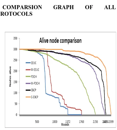
[image:14.612.297.524.71.267.2]COMPARSION GRAPH OF ALL PROTOCOLS
Figure 16 Comparison Of Number Of Nodes Alive In System Among Different Protocols
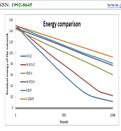
[image:14.612.319.524.349.576.2] [image:14.612.101.306.421.582.2]Figure 17 Residual Energy Comparison Among Different Protocols
[image:15.612.86.300.377.568.2]It is seen that EEUC has just 10.96J which is lowest and C-EBCP has 92.13J which is highest among all protocols.
Table 3 Comparison Table
Protocol First node dies(rounds)
Last node dies (rounds)
Residual energy after 1000 rounds in joules
EEUC 173 1372 10.96
M-EEUC
325 1763 21.84
PDCH 117 2156 59.96
M-PDCH
404 2423 76.96
EBCP 238 2453 80.75
C-EBCP 732 2598 92.13
From the table 3 proposed C-EBCP algorithm increases the time when the first node drains out of energy. It is also observed that the entire lifetime of the network i.e., the round at which the last node dies is higher for C_EBCP. This improvement is mainly due to balancing the energy consumption and effective use of chain transmission within each cluster.
6. CONCLUSION
The unequal clustering protocol EEUC and chain cluster based protocol PDCH. In both these protocols the cluster head election is made based on
the residual energy of the nodes. But by considering one more parameter i.e., distance parameter this paper proposes new method, M-PDCH for electing the cluster heads. From the simulation results it is confirmed that M-PDCH extends the life time of the network compared to PDCH. In EEUC multihop technique is used, but due to this, hot spot problem is arisen. To meet this problem, the protocol implements unequal clustering. Also the number of hops is reduced by changing the network topology in M-EEUC. But it is observed that both the rotation of cluster heads and the metric of residual energy are not sufficient to balance the energy consumption across the network. The a hybrid based EBCP protocol is introduced which balances the energy in the cluster by finding the possible position of the CH. BFO algorithm is used in finding that position. This protocol prolongs the life time of the network and reduces energy consumption when compared to other protocols. The performance of EBCP is even increased by introducing chain transmission within the clusters.
REFRENCES:
[1] I. F. Akyildiz, W. Su, Y. Sankarasubramaniam, and E. Cayirci, "A survey on sensor networks," Communications Magazine,IEEE, vol. 40, pp. 102-114, 2002.
[2] I.F.Akyildiz, W.Su, Y. Sankarasubramaniam and E. Cayirci, "Wireless sensor networks: a survey," Computer Networks,Elsevier, vol. 38, pp. 393-422, 2002.
[3] Jennifer Yick, Biswanath Mukherjee, Dipak Ghosal, "Wireless sensor network survey," Computer Networks,Elsevier, vol. 52, pp. 2292-2330, 2008.
[4] J. L.Hill, "System architecture for wireless sensor networks," University of California, Berkeley, Ph.D. dissertation 2003.
[5] G. Simon, M. Maroti, "Sensor network-based counter sniper system," in Proceedings of the 2nd international conference on Embedded networked sensor systems, Baltimore, MD, 2004, pp. 1-12.
[6] G. Tolle, D. Culler, W. Hong, et al., "A macroscope in the redwoods," in Proceedings of the 3rd international conference on Embedded networked sensor systems, San Diego, CA, 2005, pp. 51-63.
[8] P. Zhang, C.M. Sadler, S.A. Lyon, M. Martonosi, "Hardware design experiences in ZebraNet," in Proceedings of the SenSys‘04, Baltimore, MD, 2004.
[9] Welsh, K. Lorincz and M., "Motetrack: A robust, decentralized approach to RF-based location tracking," Personal and Ubiquitous Computing,Springer, vol. 11, pp. 489-503, 2007.
[10] D.J. Baker, A. Ephremides, "The architectural organization of a mobile radio network via a distributed algorithm," Transactions on Communications,IEEE, vol. 29, no. 11, pp. 1694-1701, 1981.
[11] C.R. Lin, M. Gerla, "Adaptive clustering for mobile wireless networks," Journal on Selected Areas Communications,IEEE, vol. 15, no. 7, pp. 1265-1275, 1997.
[12] K. Xu, M. Gerla, "A heterogeneous routing protocol based on a new stable clustering scheme," in Proceeding of IEEE Military Communications Conference, vol. 2, Anaheim,CA, 2002, pp. 838-843.
[13] C. C. Chiang and M.Gerla, "Routing and Multicast in Multihop Mobile Wireless Networks," in Proceedings of 6th International Conference on Universal Personal Communications, vol. 2, 1997, pp. 546-551. [14] L. Jiang, J. Y. Li, and Y. C. Tay, Cluster Based
Routing Protocol, 2004, draft-ietf-manet-dsr-10.txt,work-in-progress.
[15] M. Chatterjee, S. K. Das and D. Turgut, "WCA: A Weighted Clustering Algorithm for Mobile Ad Hoc Networks," Cluster computing,Springer Netherlands, vol. 5, pp. 193-204, April 2002.
[16] J. Y. Yu and P. H. J. Chong, "A survey of clustering schemes for mobile ad hoc networks," Communication Surveys and Tutorials,IEEE, vol. 7, no. 1, pp. 32-48, 2005. [17] M. Younis K.Akkaya, "A survey on routing
protocols for wireless sensor networks," Ad Hoc Networks, vol. 3, no. 3, pp. 325-349, 2005.
[18] A.A Mohamed, Y. Abbasi, "A survey on clustering algorithms for wireless sensor
networks," Computer communications,Elsevier, vol. 30, pp. 2826-
2841, october 2007.
[19] Q. Li and J. Aslam and D. Rus, "Hierarchical Power-aware Routing in Sensor Networks," in
Proceedings of the DIMACS Workshop on Pervasive Networking, 2001.
[20] D. Braginsky, D. Estrin, "Rumor routing algorithm for sensor networks," in Proceedings of the First Workshop on Sensor Networks and Applications (WSNA), Atlanta, 2002.
[21] C. Intanagonwiwat, R. Govindan, and D. Estrin, "Directed diffusion: a scalable and robust communication paradigm for sensor networks," in Proceedings of the 6th annual international conference on Mobile computing and networking, 2000, pp. 56-67.
[22] C. Rahul, J. Rabaey, "Energy Aware Routing for Low Energy Ad Hoc Sensor Networks," in Wireless Communications and Networking Conference,IEEE, vol. 1, 2002, pp. 350-355. [23] W.Heinzelman, A.Chandrakasanand and H.
Balakrishnan, "Energy-efficient communication protocol for wireless microsensor networks," in Proceedings of the 33rd Annual Hawaii International Conference on System Sciences, Maui, HI, 2000, pp. 3005-3014.
[24] W.B. Heinzelman, A.P. Chandrakasan, H. Balakrishnan, "Application specific protocol architecture for wireless microsensor networks," Wireless Communications,IEEE, vol. 1, pp. 660-670, october 2002.
[25] S. Lindesy and C. Raghavendra, "PEGASIS: Power-Efficient Gathering in Sensor Information System," in Proceedings of the Aerospace Conference,IEEE, vol. 3, Big Sky, Montana, 2002, pp. 9-16.
[26] A.W. Krings Z. (Sam) Ma, "Bio-Inspired Computing and Communication in Wireless Ad Hoc and Sensor Networks," Ad Hoc Networks,Elsevier, vol. 7, no. 4, pp. 742-755 , June 2009.
[27] S. Selvakennedy, S. Sinnappan, Yi Shang, "A biologically-inspired clustering protocol for wireless sensor networks," Computer Communications,Elsevier, vol. 30, pp. 2786-2801, 2007.
[28] Chao Wang and Qiang Lin, "Swarm intelligence optimization based routing algorithm for Wireless Sensor Networks," in proceedings of International Conference on Neural Networks and Signal Processing, 2008, pp.