"SIMULATION OF OXYGEN DYNAMICS RELATIVE TO PURIFICATION OF FRESH WATER" by
R. L. Wilson INTRODUCTION
This study describes the simulation, on both the PACE®.TR-48 and TR-20 desk-top general pur-pose analog computers, of the basic forces affect-ing the condition of fresh water sewage receivers ... biochemical oxygen demands from sewage decom-position and free oxygen content in the receiving waters ... and an investigation as to how the re-. sulting dynamic sewage load/oxygen relationship
determines, to a great extent, the increasingly important, and often confused, "water pollution status" of the country's rivers, lakes and streams.
In the decomposition of the bulk of sewage com-ponents, whether from domestic or industrial
sources, oxidation plays an important role. It is recognized, of course, that without exhaustive data regarding particular receiving waters nothing ap-proaching a complete discussion of the oxygen dynamics of fresh and saline water would be pos-sible. The purpose of this simulation is to examine these basic forces in general and to show how they can be simulated with some degree of sophis-tication on small, general purpose computers. The techniques used then can be extended for use in model building programs with data obtained for specific bodies of water. In this more sophisticated area of simulation, significant strides of real
economic and educational value can result. BENEFITS
Several benefits are provided by this simulation not only in terms of offering greater insight into the dynamics of water pollution, but also in provid-ing basic data for more advanced and sophisticated analyses (such areas are delineated later).
The entire area of water pollution and waste water treatment is receiving increasingly greater atten-tion by the general public as well as by federal and international government agencies. Detergent deg-radation of water supplies generally, and the Great Lakes/City of Chicago water diversion controversy
in particular, are only two of the more publicized aspects of the overall problem.
Through the analog computer simulation of the
relatively simple oxygen dynamics of fresh and saline waters, significant information is obtained
1
for laboratory use in determining the important parameters of receiving waters ... percentage and type of organic waste, diffusion and discharge patterns, etc. Through curve matching techniques involving dissolved oxygen depletion, effluent rate pattern and strength, reoxygenation rate, etc., it is possible to obtain the "book" on speCific bodies of receiving water, which is useful in formulating basic design criteria for the construction and opera-tion of water treatment plants.
PROBLEM DISCUSSION
The basic goals of modern sewage treatment plants can be summarized as follows:
1. to remove the larger and more objectionable settleable solids through screening and sedi-mentation,
2. to reduce the effluent "load" on the receiving waters to reduce stream degradation to a reasonable level and then maintain it, and 3. to operate efficiently in terms of initial
in-vestment and operating costs.
Current design and operation to achieve these goals range from ultra-sophisticated activated-bacterio-logical treatments to simple, short-duration hold or settling tank procedures.
Enormous economies can be achieved in the design and operation of municipal and industrial sewage treatment plants through the proper interpretation of data concerning the oxygen dynamics of water supplies. The effectiveness of these plants, of course, will determine then the design, operation and associated costs of related water intake treat-ment plants and, ultimately, overall water quality for all uses.
For a clear understanding of the entire pollution/ treatment problem in terms of oxygen dynamics, and for the necessary critical evaluation of existing
facilities, it is paramount to recognize that the
re-ceiving water itself is the final stage of sewage
treatment, the initial steps being the formal treat-ment plant. This final stage, utilizing the self-purification properties of the water, must be as
carefully analyzed and managed as the plant itself.
!c) Electronic Associates, Inc. 1964
Indeed, in the absence of any real, formal treatment plant, the receiving waters are often the only stage of water treatment and their analysis and manage-ment become even more critical.
If oxygen conditions in streams receiving treatment
effluent are kept within certain limits, the capacity of these streams to digest enormous sewage loads without adverse pollution effects truly is amazing. On the other hand, if oxidation cannot occur because of overloading or other factors, a septic stream is
the result. If oxygen depletion is too great, the
degree of pollution can range from unfit drinking water through the destruction of wildlife resources and water unfit for bathing to even water unfit for raw industrial use.
Figure 1 shows graphically the relationship between oxygen deficit and septic stream conditions.
o
TIME FROM INTRODUCTION OF SEWAGE LOAD~ o
a::
u. DANGER LEVEL
t
_
D NON POTABLE LEVELSiL C SEPTIC LEVEL
~ - - - 1 0 0 % 0 2 DEPLETION
[image:2.615.60.569.240.721.2]NO
Figure 1: Curve Showing Relationship Between Oxygen Deficit & Stream Degradation
D1
=
Initial Deficit. Dc=
Critical Deficit D2 = Recovery Deficit (D changes sign)The problem, then, is to determine not only the oxygen content of particular receiving waters but also to analyze the factors which cause oxygen depletion, .and to discover sources which either by themselves or through dynamic interaction with others can help to replenish the dissolved oxygen supply.
PROBLEM ANALYSIS
Two basic influences determine the degree of oxygen depletion and pollutional degradation of a receiving water: the capacity it has for oxidizing organic sew-age components, as measured by the amount of dis-solved oxygen contained per unit volume of the water, and the demands made on it for oxygen by such components, as measured by the Biochemical
Oxygen Demand (BOD) per unit volume. t
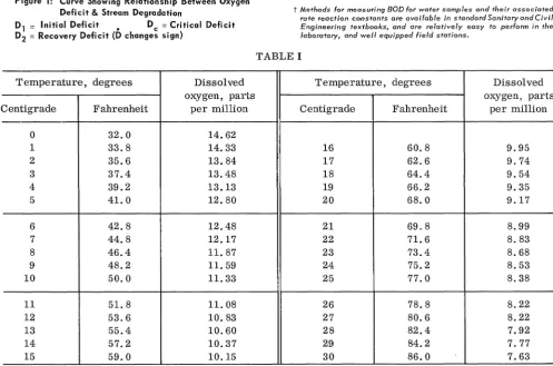
Water normally contains oxygen in solution in varying percentages depending on 'freshness' and temperature. Saturation values are obtained from true fresh water samples -- rain water, mountain streams, waterfalls, etc. Table 10shows typical values of oxygen saturation in fresh water samples at different temperatures. The values for saline (seawater) samples are approximately 80 per cent of the fresh water values and are similarly temperature-variant.
As this dissolved oxygen in the receiving water is used to supply the oxidation demands of the sewage BOD, additional oxygen must be obtained either from
t Methods for measuring BOD for water samples and -their associated rate reaction constants are avaifable in standard Sanitary and Civil Engineering textbooks, and are relatively easy to perform in the
laboratory, and well equipped field stations.
TABLE I
Temperature, degrees Dissolved Temperature, degrees Dissolved
oxygen, parts oxygen, parts
Centigrade Fahrenheit per million Centigrade Fahrenheit per million
0 32.0 14.62
1 33.8 14.33 16 60.8 9.95
2 35.6 13.84 17 62.6 9.74
3 37.4 13.48 18 64.4 9.54
4 39.2 13.13 19 66.2 9.35
5 41. 0 12.80 20 68.0 9.17
6 42.8 12.48 21 69.8 8.99
7 44.8 12.17 22 71. 6 8.83
8 46.4 11. 87 23 73.4 8.68
9 48.2 11. 59 24 75.2 8.53
10 50.0 11. 33 25 77.0 8.38
11 51. 8 11. 08 26 78.8 8.22
12 53.6 10.83 27 80.6 8.22
13 55.4 10.60 28 82.4 7.92
14 57.2 10.37 29 84.2 7.77
15 59.0 10.15 30 86.0 7.63
[image:2.615.62.560.387.716.2]the atmosphere (via aeration) or from other bodies of water rich in oxygen (via stream diversion) to make up the deficiency.
A. Aeration: When using atmospheric reaera-tion, the rate of oxygen renewal in the water
varies with 1.) The amount of oxygen deficit
measured from saturation value (which is temperature-variant and, hence, subject to seasonal changes as well as day to day ambient
temperature conditions), and 2.) The degree of
physical intermixing of atmosphere and water possible for a particular stream flow and con-figuration (commonly dependent upon the geo-metric shape of the body of water, its velocity, surface wind action, wave action, and turbulence such as waterfalls, rapids, etc.).
The classic example of artifiCially inducing a greater mixing of water and atmosphere is the aeration of the Flambeau River at Park Falls, Wisconsin.
B. Stream Diversion: The classic example of using water richer in oxygen to provide the necessary dissolved oxygen to a stream to pre-vent septic stream condition is the diversion of
Lake Michigan by the City of Chicago to flow down the IllinoiS and Des Plaines rivers.
It should be noted that both of these programs were relatively successful despite their
contro-versial aspects. In each case, their use postponed
necessary improvements in existing treatment plants and their relative success in providing re-oxygenated water permitted considerable savings in plant investment.
In terms of the overall problem of waste water
treatment, however, the successful application of such artificial means -- means not involving formal treatment plants, as such -- illustrates clearly that the task of water purification can be handled quite well by efficient management of oxygen dynamics alone.
SYSTEM EQUATIONS
The relationship existing among the various factors involved in oxygen dynamics can be expressed in the following greatly Simplified differential equation commonly called the Oxygen Sag Equation:
dD
- = k (L -y) -r D
dt a
where D = oxygen deficit, mg/l
D. = oxygen deficit at time t = 0
1
k = BOD rate coefficient
La = BOD load, mg/l
(1)
y = total BOD load exerted in time t, mg/l
r = reoxygenation rate coefficient
t = time measured from introduction of
La
The variable y can be defined further by the follow-ing expression:
kt Y = La (1 - e )
Ck (T - To)
where k = k e
also
and
o
r = r e o
C (T - To) r
CL (T - To)
L a = L e
0
T = water temperature, deg. C
(2)
T = base temperature for determination of
o
ko' ro and Lo' deg. C.
e = natural log base
The values Ck, C rand CL are "empiricized" coefficients unique to
1.) flow rate pattern
2.) percentage salinity
3.) percentage inorganic waste and type
4.) type of organic waste
5.) extent of plant life and normal daily and annual
cycle
6.) extent of "sludge" deposits (past history of stream)
7.) profile of receiving water (surface area vs,
profile areas)
8.) wave action in water
9.) turbulence of flow
10.) surface wind phenomena
11.) tidal action
12.) pattern of sewage diffusion
13.) pattern of sewage discharge.
These thirteen characteristics are those with which the more serious examinations of water/
oxygen dynamics are concerned, Outstanding
of these parameters (to reduce the empirical representation of them) and many advanced studies currently are being carried out with the aid of large and quite sophisticated analog computer
programs. t
It should be noted, however, that this general
expression Equation (1) of the Oxygen Sag Equa-tion is derived per unit of receiving water volume.
It should not be confused with the ultimate total
digestion capacity of a stream since flow varia-tion and diffusion patterns play an important role
in determining this ultimate value. This is
particularly true where the receiving waters are lakes, bays, estuaries or streams with
unpredic-table or highly variant flows. t For many
ap-plications, however, involving receiving waters not subject to such physical disturbances, the general Oxygen Sag Equation is descriptive of the typical oxygen/water balance existing.
One additional coefficient that is encountered oc-casionally in the analysis of oxygen dynamics is f, referred to as the self-purification constant, which can be expressed as®
f =r/k (3)
This value provides a rough estimate as to a receiving water's ability to "cleanse" itself. Table II shows typical order-of-magnitude values of f for various types of receiving waters.® Figure II shows the variations of k and r with
temperature for a particular stream.
CD
TABLE II
Typical Values of f at 20°C
Small ponds & backwaters . . . . Sluggish streams, Large lakes.
Large streams of low velocity .
0.5-1. 0
1.0-1.5
1. 5-2. 0
Large streams of moderate velocity . .. 2. 0-3. 0
Swift streams . . . 3.0-5.0
Rapids and waterfalls . . . .. above 5
It can be seen that even though the value of f,
itself, decreases with increase in temperature (because of increasing BOD rate), the accompany-ing rise in reoxygenation rate shows that warm water can recover oxygen in solution more quickly
than cool water. This basic characteristic of
oxygen dynamics can be used effectively in en-hancing the efficiency of treatment plants either by increased utilization of artificial heating means or more sophisticated employment of ambient
temperature ranges in the receiving water.
t Typical of the advanced work being done in this area is the study entitled "Analog Computation of the Dispersion of Pollutants in the Delaware Estuary" by Dr. J. O'Connor, L. L. Folk, and RI G.
E. Franks
c,j 2.0
f1i
o
~ 1.0
... O.B ex .joJ 0.6 ;:) 0.5
..I
~ 0.4 0.3
1..0""
---5
~
~ r~-
RELATION BETWEEN VALUES OF K DEOXYGENATION COEFFICIENT AND OF RE-AERATION COEFFICIENTr
AT 20 DEGREES CENTIGRADE AND VALUES AT OTHER I TEMPERATURES ~o 0.2
~ 5 10 15 20 25 30 35
0: TEMPERATURE,DEG. C.
Figure 2: Relation Between k and rat VariCilus Temperatures
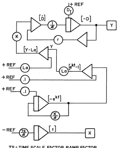
ANALOG SIMULATION PROGRAMS
The analog computer programs used to simulate the dxygen Sag Equation are straight-forward. Three of these programs, illustrating the various degrees of sophistication possible and the various complement of hardware required, are presented
unscaled in Figures 3, 4 and 5. A completely
scaled and working diagram for the circuit shown in Figure 4 is shown in Appendix A.
[ t]
.>=--=---1 X
TS = TIME SCALE FACTOR RAMP FACTOR
Figure 3: Straightforward Mechanization of Basic Oxygen Sag Equation
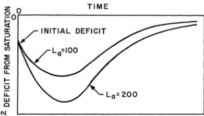
RESULTS
Typical of the results obtained are the curves
shown in Figures 6 and 7. Figure 6, obtained
[image:4.612.317.553.45.167.2] [image:4.612.339.537.350.596.2]REF
+
REF - REF+
REF.1
-REF-QD~---~IT>---~
TS: TIME SCALE RAMP FACTOR
Figure 4: Use of Multipliers to Enoble Coefficients, k ond La' to be Set on Single Potentiometers
To: CONSTANT
-10
+10
+10 I
I
---'
+10 I
I
_ _ _ _ _ _ _ _ _ ...J
6 POTS 12 AMP
3 ± LOG FUNCTION GEN.
+K
or-K
TO CIRCUIT IN FIG 4. REPLACES VALUE OF K SET ON POT.
TO CIRCUIT IN FIG 4. REPLACES VALUE OF r SET ON POT. ADDITIONAL MULTIPLIER REQUIRED IN FIG 4.
TO CIRCUIT IN FIG 4. REPLACES VALUE OF La SET ON POT.
[image:5.620.88.511.39.347.2] [image:5.620.84.521.383.692.2]where La was the variable parameter, illustrates the time required for a constant-temperature re-ceiving water to replenish its dissolved oxygen content after various BOD requirements.
Figure 7, obtained from runs of the computer cir-cuit of Figure 4, shows similar dissolved-oxygen vs. time curves for receiving water at several dif-ferent temperatures.
TIME
Z 0
Qo~---~ ~ 0: ;:) ~ (f) ~ o 0: IL l-t:) ii: w o N o
Figure 6: Effect of Various BOD Loads on Dissolved Oxygen Recovery Time. Temperature Constant
z TIME
o~---~
fi
0: ;:) ~ (f) ~ o 0: IL l-t:) IL W o N oFigure 7: Effect of Various Temperatures on Dissolved Oxy. gen Recovery Time, BOD Load Constant
Briefly summarized, the following observations can be made regarding the results obtained from this
study:
1. With a constant BOD load -- e.g. regular as
opposed to intermittent bulk discharges of sewage or waste, etc. -- the higher the tem-perature of the receiving water, the more
rapid and the more complete the depletion of dissolved oxygen from that water, but the quicker the recovery rate of oxygen back into solution.
2. With a constant temperature, the higher the load the more rapid and complete the deple-tion of dissolved oxygen, as above, and again the quicker the recovery rage.
3. A significant area of optimization exists as to loading vs. temperature, particularly in
re-gard to effluent rate pattern and strength. In
this regard, Figure 1 illustrates several im-portant criteria of the oxygen deficit curve.
4. Where measurements have been made from field samples, it is possible by curve matching to determine several important characteris-tics of the receiving water, such as reoxygena-tion rate coefficient at base temperature, ro, BOD rate coefficient at base temperature,
ko,
and value of self-purification constant atbase temperature, fo, as well as those aspects of water/oxygen dynamics relative to salinity, plant life, organic and inorganic waste, etc., (Ck, Cr , CL)· These characteristics then can be related to ambient temperature ranges in the receiving water.
This method of curve matching makes it possible to obtain the "book" on a particular body of re-ceiving water and to use this complete oxygen dynamics analysiS as basic design criterion for the construction and operation of a treatment plant.
This method of curve matching makes it possible to obtain the "book" on a particular body of re-ceiving water and to use this complete oxygen dynamics analysis as basic design criterion for the construction and operation of a treatment plant.
CONCLUSION
This analog computer simulation of relatively sim-ple oxygen dynamics offers several important ad-vantages. Educationally, it provides an insight into stream pollution itself that has not been completely available in the past by giving anew look at the fac-tors both effecting and affecting such pollution.
In the laboratory, the simulation can be put to use
in rapidly determining the important parameters of receiving waters either to form the basis for selection or rejection of a particular body of water or to provide information as to the amount of pre-conditioning necessary in the water to meet the requirements of projected sewage loads.
Of the utmost importance, however, is the fact that this simulation, which can be performed with a fair degree of sophistication on a small, general purpose analog computer, provides a convenient and inexpensive means to obtain complete oxygen
dynamics analyses. This data, properly
[image:6.620.76.284.168.286.2] [image:6.620.75.286.359.480.2]APPENDIX A
Computer Mechanization of Oxygen Sag Equation
dD
ill
= k (La - y) -r D (1)where y = L (1 _ ekt)
a
Conversion Factors
1 ppm
D.
1
= 1 mg/liter - 8.34 lb/million gallons
= 3 mg/liter (max. assumed)
D
mx = 15 mg/liter (max. assumed)
= 500 mg/liter (max. assumed,
theo-retically unlimited)
La' typical = 20-400 mg/liter
y, max. = 500 mg/liter (max. assumed,
theo-retically unlimited)
y, typical = 200-400 mg/liter
k, typical = 0.25-0.75/ day
r, typical = 0.25-1.00/day
+10 +10
10
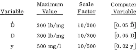
Scale Factors
Maximum Scale Computer
Variable Value Factor Variable
D 200 Ib/mg 10/200 [0.05 DJ
D 200 lb/mg 10/200 [0.05 DJ
y 500 mg/I 10/500 [0.02 yJ
The potentiometer sheet is shown in Table III.
The scaled computer diagram is shown in Fig-ure 8.
TABLE III
Pot Sl S2 S3 S4 Parameter
1 .8 .8 .6 .6 K
2 .1 .1 .1 .1 Di
3 .100 .125 .125 .125 La
4 .7 .7 .5 .7 r
5 CONS TANT .25
6 CONS TANT .20
7 CONS TANT .1
8 CONS TANT 1.0
9 CONS TANT .5
20 TIME BASE GENE RATOR .065
-10 +10
7
-10
-"-@I---[B>'---[]
[image:7.615.312.544.56.141.2]BIBUOGRAPHY
1. Urquhart, L. C.: Civil Engineering Handbook, McGraw-Hill, New York, 1959.
2. Fair, G. M., and J. C. Geyer: Water Supply and Waste Water Disposal, John Wiley & Sons, Inc.,
New York, 1954.
EAI
OELECTRONIC ASSOCIATES, INC. West