Identification, estimation and efficiency of nonparametric and semiparametric models in microeconometrics

Shiisn utnwv ^ Wt o*

Id en tification , E stim a tio n and

E fficiency o f N on p aram etric and

Sem iparam etric M od els in

M icroeconom etrics

David Tomas Jacho-Chavez

A D issertation su b m itted to th e D epartm ent of Econom ics in p a rtia l fulfilment of the requirem ents for th e degree of

Doctor of Philosophy

London School of Economics and Political Science

UMI Number: U 213529

All rights reserved

INFORMATION TO ALL U SE R S

The quality of this reproduction is d ep en d en t upon the quality of the copy subm itted.

In the unlikely even t that the author did not sen d a com plete m anuscript

and there are m issing p a g e s, th e se will be noted. Also, if material had to be rem oved, a note will indicate the deletion.

Dissertation Publishing

UMI U 213529

Published by ProQ uest LLC 2014. Copyright in the Dissertation held by the Author. Microform Edition © ProQ uest LLC.

All rights reserved. This work is protected against unauthorized copying under Title 17, United S ta tes C ode.

ProQ uest LLC

789 East E isenhow er Parkway P.O. Box 1346

D eclaration

I hereby declare:

• No p a rt of this doctoral dissertation has been presented to any University for any degree.

• C hapter 2 was undertaken as joint work w ith Professor Oliver B. Linton and Professor A rthur Lewbel.

~ T H £ i S E s

A b stract

The focal point of this thesis is on identification and estim ation of nonparam etric models, as well as the efficiency and higher order properties of a class of sem iparam etric estim ators in Microeconometrics.

We present a new identification result for a particular nonparam etric model th a t nests many popular param etric/ nonparam etric Econom etric models as special cases. Estim ators are proposed and their asym ptotic properties derived; in particular, they axe shown to be consistent and asym ptotically pointwise normally distributed. We im plem ent these estim a­ tors for the nonparam etric estim ation and testing of production functions in 4 industries within the Chinese economy in the years 1995 and 2001.

The statistical properties of an entire family of sem iparam etric estim ators for Limited Dependent Variables models are also analyzed. The derived theoretical results have direct applicability to a wide range of estim ation problems. In particular, we derive the sem ipara­ m etric efficiency bounds and show th a t some of the already-proposed estim ators achieve these bounds. A connection w ith the Program m e Evaluation literature is established as well.

Table o f C on ten ts

T a b le o f C o n t e n ts 4

L is t o f F ig u r e s 6

L is t o f T a b le s 7

1 I n t r o d u c t i o n 9

2 I d e n tif ic a tio n a n d N o n p a r a m e tr i c E s tim a tio n o f a T r a n s f o r m e d A d d itiv e ly

S e p a r a b le M o d e l 12

2.1 In tro d u c tio n ...12

2.2 I d e n tif ic a tio n ... 15

2.3 E stim ation ...19

2.4 A sym ptotic P r o p e r t ie s ...22

2.5 Num erical R e s u l t s . ... 26

2.5.1 S im u la tio n s ...26

2.5.2 Generalized Hom othetic Production Function E s t i m a t i o n ... 29

2.6 Conclusion and Extensions ... 37

2.A M ain P r o o f s ...40

2.B Technical L e m m a s ... 49

2.C Tables &; F i g u r e s ...67

3 E ffic ie n c y B o u n d s in S e m ip a r a m e tr ic M o d e ls d e fin e d b y M o m e n t R e s t r i c ­ tio n s u s in g a n E s t im a t e d C o n d itio n a l P r o b a b il it y D e n s ity 85 3.1 I n tro d u c tio n ... 85

3.2 Efficiency and In fo rm a tio n ...88

3.3 Some Efficiency B o u n d s ...91

3.3.1 Model 1 ... 91

3.3.2 Model 2 ... 93

3.3.3 Model 3 ... 94

3.4 A M onte Carlo Investigation ... 95

Table of Contents

3.A M ain P r o o f s ... 99

3.B T a b l e s ... 106

4 O p tim a l B a n d w id t h C h o ic e fo r E s t im a t i o n o f I n v e r s e C o n d itio n a l—D e n s i ty - W e ig h te d E x p e c ta t io n s 116 4.1 In tro d u c tio n ... 116

4.2 A sym ptotic Mean Square E r r o r ... 118

4.2.1 F r a m e w o r k ...118

4.2.2 Sensitivity Analysis ...121

4.2.3 ‘N onparam etric’ vs ‘Sem iparam etric’ O ptim al B a n d w id th s ...124

4.3 O ptim al ‘p lu g -in ’ B andw idth E s t i m a t o r ... 125

4.4 M onte Carlo E x p e r im e n ts ... 128

4.5 E x te n sio n s... 131

4.5.1 Mixed Continuous and Discrete C a s e ... 131

4.5.2 B andw idth Selection using the ra-o u t-o f-iV B o o t s tr a p ... 134

4.6 Conclusion ... 135

4.A M ain P r o o f s ... 137

4.B Technical L e m m a s ...166

4.C Tables &; F i g u r e s ... 185

List o f Figures

2.1 Q — Q plots for G, F and H... 74

2.2 Simulation Envelopes for M , G and F... 75

2.3 Generalized Hom othetic Translog Isoquants... 76

2.4 Generalized Homogeneous M ( 1 9 9 5 ) ... 77

2.5 Generalized Homogeneous Component G(1 9 9 5 )... 78

2.6 Generalized Homogeneous Com ponent F (1 9 9 5 )... 79

2.7 Strictly M onotonic Component H (1995)... 80

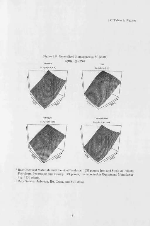
2.8 Generalized Homogeneous M ( 2 0 0 1 ) ... 81

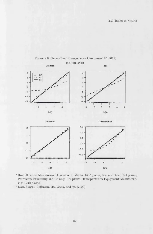
2.9 Generalized Homogeneous Component G(2 0 0 1 )... 82

2.10 Generalized Homogeneous Component F (2 0 0 1 )... 83

2.11 Strictly M onotonic Com ponent H (2001)... 84

4.1 V isualization of Design 1... 192

4.2 V isualization of Design 2 ... 193

4.3 V isualization of Design 3 ... 194

4.4 Sim ulated M S E of Design 1 ...195

4.5 Sim ulated M S E of Design 2 ...196

List o f Tables

2.1 M edian of M onte Carlo fit criteria over grid for Design 1. . . . ! ...68

2.2 M edian of M onte Carlo fit criteria over grid for Design..2... 69

2.3 P aram etric General Production Function E stim ates ( P I ) ... 70

2.4 P aram etric Generalized Hom othetic Estim ates ( P 2 ) ... 71

2.5 P aram etric Translog Estim ates ( P 3 ) ... 72

2.6 Average Substitutability, T (k, L )...73

2.7 Average R eturn to Scale, R T S (M , L) ...73

3.1 M onte Carlo results for Design 1 ... 107

3.2 M onte Carlo results for Design 1 ... 108

3.3 M onte Carlo results for Design 1 ... 109

3.4 M onte Carlo results for Design 2 ...110

3.5 M onte Carlo results for Design 2 ...I l l 3.6 M onte Carlo results for Design 2 ...112

3.7 M onte Carlo results for Design 3 ...113

3.8 M onte Carlo results for Design 3 ...114

3.9 M onte Carlo results for Design 3 ...115

4.1 M onte Carlo results for Design 1: B andw idth E stim ation ...186

4.2 M onte Carlo results for Design 1: Param eter r j ...187

4.3 M onte Carlo results for Design 2: B andw idth E stim ation ...188

4.4 M onte Carlo results for Design 2: Param eter t j ...189

4.5 M onte Carlo results for Design 3: B andw idth E stim ation ... 190

A cknow ledgem ents

I would like to extend my most sincere thanks and appreciation to my supervisor, Oliver Linton, for his support, priceless advice and patience. Oliver’s optim ism and good humour were always very helpful during the completion of this dissertation. His valuable insights were crucial for this work. I will always consider myself incredibly fortunate to have worked under his supervision.

Jezam in Lim, my partner, deserves special mention. She has been my inspiration and source of strength during good and bad times. Her love, understanding and support have made this dissertation possible. I will be forever in debt w ith her.

Throughout my higher education, I have received financial support from the D epartm ent of Economics a t the London School of Economics and Political Science, and the Escuela Superior Politecnica del Litoral (Ecuador). Many thanks goes to everyone a t these places.

Chapter 1

In trod u ction

Nonparam etric and sem iparam etric specifications are common in Econom etric models. In Microeconomics, they are informative about consumer or firm behavior while imposing a minimum set of restrictions in order to achieve identification of the m ain features of interest. Furtherm ore, non/sem ipaxam etric econometric estim ators can be constructed (in some cases efficiently) to rem ain consistent in situations where param etric models are not. This robustness property rem ains the most im portant aspect in this literature.

The calculation of fully nonparam etric estim ators, while m odeling economic relation­ ships, imposes enorm ous d a ta requirem ents when a large num ber of variables is involved. This problem, known as the ‘curse of dim ensionality’, can be alleviated by the use of cer­ tain functional structures th a t may be imposed by Economic theory. These nonparam etric functional forms are more restrictive th a n a fully nonparam etric specification, b u t their as­ sum ptions are weaker th a n those w ith a finite-dim ensional param etric specification. These particular forms (as we will show in this dissertation) can be used to identify the model itself, and we build estim ators th a t achieve faster rates of convergence relative to their non­ param etric counterparts. On the other hand, sem iparam etric models are also very attractive alternatives to reduce this ‘curse of dim ensionality’. They impose some param etric restric­ tions on the economic relationship th a t we try to model, while allowing functional form of many of its other com ponents to rem ain unknown. A large num ber of the derived sem ipara­ m etric estim ators achieve param etric rates of convergence, and a tta in th e sem iparam etric efficiency bounds induced by their underlying assembly.

C h a p t e r 2: I d e n tif ic a tio n a n d N o n p a r a m e tr i c E s t im a t i o n o f a T r a n s f o r m e d A d d itiv e ly S e p a r a b le M o d e l. We first introduce a flexible stru ctu re for a function of random variables th a t nests m any features of Econom etric models as special cases. This particular form involves a sm ooth monotonic transform ation of another sm ooth function, which is assum ed to be separable, either additively or multiplicatively, w ith respect to one of its argum ent. For example: This particular functional form could represent the condi­ tional m ean or quantile function of the observed outcom e in Lim ited D ependent Variable Models. It could also represent hom othetic functions widely used in Economic modeling. In a regression model w ith unknown transform ation of the dependent variable, the condi­ tional distribution of the dependent variable given the observed regressors, also shares this functional form.

Unlike other authors in this literature, we make full use of the implied strictly mono­ tonic link function in th e examples above to achieve nonparam etric identification of all their unknown components. Furtherm ore, we propose a com putationally simple nonparam etric estim ation algorithm th a t does not require any optim ization or m atching. The resulting es­ tim ators have pointwise asym ptotic norm al distributions under regularity conditions. Their rates of convergence are also faster th an those of a fully nonparam etric alternative. We also find th a t they perform fairly well in comparison w ith other nonparam etric estim ators previously proposed in the literature, for a variety of M onte Carlo designs dealing with small sample sizes.

Finally, th e idea of Generalized Hom othetic functions is introduced in order to estim ate production functions for various industries within the Chinese economy during the years 1995 and 2001. We also estim ate and test a range of param etric specifications for comparison purposes. In certain industries, we find th a t their implied m easures of input substitution and scale are very different to those implied by our more flexible specification.

C h a p t e r 3: E ffic ie n c y B o u n d s in S e m ip a r a m e tr ic M o d e ls d e fin e d b y M o m e n t R e s t r i c ti o n s u s in g a n E s t im a t e d C o n d itio n a l P r o b a b il it y D e n s ity . In this chapter, we calculate th e sem iparam etric efficiency bounds for an entire class of sem iparam etric estim ators proposed in th e literature of Limited D ependent Variable models. Regardless of the inherent nonlinearities of this type of model, these estim ators are com putationally easy to calculate as they have ‘closed’ formulae. In some cases, they resemble Least Squares or Linear Instrum ental Variable estim ators in a simple linear regression model. They are also robust to m easurem ent errors, endogeneity and heteroskedasticity of unknown form.

probability density in the construction of these estim ators is more efficient. Furtherm ore, the general result presented in this chapter can be directly applied to any new estim ator th a t belongs to this class. All these results seem to be new in the literature.

Our theoretical findings are confirmed in a sim ulation stu d y involving a variety of designs, frameworks and kernel-based estim ators. We find m arginal improvements in term s of fitting criteria when Local Linear instead of Local C onstant regression is used for the nonparam etric component of th e estim ator.

C h a p t e r 4: O p tim a l B a n d w id th C h o ic e fo r E s t im a t i o n o f I n v e r s e C o n d itio n a l- D e n s ity - W e ig h te d E x p e c ta tio n s . The kernel-based im plem entation of the class of semi­ param etric estim ators discussed in C hapter 3 requires th e choice of a sm oothing param eter. This chapter characterizes its optim al value. We obtain a ‘closed’ formula for the optim al bandw idth by minimizing the leading term s of a second-order m ean squared error expansion of the estim ator w ith respect to this sm oothing param eter.

It tu rn s out th a t we can choose the optim al value for th e bandw idth based on bias alone. In particular, we show th a t there are two sources of biases: a ‘sm oothing’ bias, and a ‘degrees-of-freedom ’ bias. The optim al bandw idth makes these biases’ contributions to the asym ptotic m ean square error have the same order of m agnitude. Based on the derived formula for the optim al smoothing param eter, a simple ‘p lu g -in ’ estim ator for the optim al bandw idth is proposed. We prove its consistency under regularity conditions.

We exam ine th e quality of the asym ptotic approxim ation in finite samples for simple Monte Carlo designs. The proposed ‘plu g -in ’ estim ator for th e optim al bandw idth is also shown to perform fairly well under various circum stances and sample sizes. Finally, we examine how our results ad apt in the presence of discrete regressors. T he potential use of a B ootstrap bandw idth selection mechanism is also presented.

Chapter 2

Id en tification and N on p aram etric

E stim a tio n o f a Transform ed

A d d itiv ely Separable M od el

2.1

In tr o d u ctio n

For vector x and scalar z, let r (x, z) be a function th a t, along w ith its derivatives, can be consistently estim ated nonparametrically. U nconstrained nonparam etric estim ation of r is usually u n attractiv e when x € is m ultidimensional, because the ra te of convergence decreases rapidly as d increases, yielding very imprecise estim ates w ith samples of practical size, see Stone (1980). We may overcome this curse of dim ensionality by making assum p­ tions about the functional form of r th a t are stronger th an those of a fully nonparam etric estim ator, b u t weaker th a n those of a finite-dim ensional param etric model, see Stone (1986). In the fully nonparam etric framework, one such dim ension-reduction m ethod is to assume there exist functions iif, G and F such th a t

2.1 Introduction

This framework encompasses a large class of economic models. For example, the func­ tion r (x, z) could be utility or consumer cost functions recovered from estim ated consumer dem and functions via revealed preference theory, or it could also be a production or pro­ ducer cost function th a t can be recovered directly from a d a ta set. W hen H [m] = m, the identity function, Chiang (1984), Simon and Blume (1994), B airam (1994), and Chung

(1994) reviewed popular param etric functional forms used in economics. In dem and analy­ sis, Goldm an and Uzawa (1964) provideed an overview of the variety of separability concepts implicit in such specifications.

M any m ethods have been developed for the identification and estim ation of strongly or additively separable models, where r (x, z) = Yl t =i @k (%k) + F (z) or its generalized version r ( x , z) = # E j t = i Gk {%k) + ^ (2:)]. Friedm an and Stutzle (1981), Breim an and Friedm an (1985), Andrews (1991), Tjpstheim and A uestad (1994) and Linton and Nielsen (1995) are examples of the prior and Linton and Hardle (1996), and Horowitz and Mammen (2004) proposed estim ators of the latter for known H. Horowitz (2001) used this assumed strong separability in order to identify the components of the model when H is entirely unknown, and proposed a kernel-based consistent and asym ptotically norm al estim ator. W hen d — 1, specification (2.1.1) is nested in the class of models Horowitz considers. However, m any econometric models imply link functions, H , th a t are strictly monotonic b ut otherwise unknown (see examples below). By m aking use of this ex tra information, our identification result does not requires G to be additive in its argum ent, in order to achieve full identification.

As strong separability may be too restrictive in th e context of an empirical application, models satisfying equation (2.1.1) axe called weakly separable. They offer a more flexible specification th a t allows for some interaction among regressors, as well as a faster rate of convergence com pared to fully unrestricted nonparam etric estim ation. Pinkse (2001) provides a general nonparam etric estim ator for this class of models under weaker conditions on M , i.e. no separability, and on H, which is assumed to be increasing only. However, in this partly separable specification, Pinkse’s estim ator will com pute M up to an arbitrary monotonic transform ation; while ours, by making use of th e assum ed strict m onotonicity of H, provides the unique (up to sign-scale and location norm alization) M , and by virtue of m arginal integration, the unique G and F.

2.1 Introduction

in particular are commonly of this form, having Y = 1 [G (X ) + e > —z], where — z is some threshold, e.g. price or bid, with G ( X ) + e being willingness to pay. In this sense, our identification result is similar to Lewbel and Linton (2002) for the censored or truncated regression, though it is applicable to a wider range of Lim ited D ependent Variable models, and makes use of the extra assumed separability.

Model (2.1.1) m ay also become evident in a regression m odel w ith unknown transfor­ m ation of the dependent variable, F (z) = G (x) + £, where e has absolutely continuous distribution function H which is independent of x, F is an unknown m onotonic transfor­ m ation and G, an unknown regression function. It follows th a t th e conditional distribution z given rr, F z \ x> is given by H ( F {z) — G( x ) ) = r (z, x), where F z \ x = r (z >x )- For this model, Ekeland, Heckman, and Nesheim (2004) provided an identification result th a t also exploits separability between x and z, b u t not the m onotonicity of H as we do here. More generally, M atzkin (2003) considered identification of models of the form Y = m (X, Z, e) with e independent of ( X, Z). In this framework, our model makes no assum ption about the role of unobservables, as well as provides no estim ates of these other th an a limiting distribution theory for estim ates of r.

Moreover, th e proposed identification result may also be extended to th e transform ed m ultiplicative sub-m odels of the form H [M (x, z)\ = H [G (x) F (z)], which are very com­ mon in production literature. Particularly, a function r (x, z) is said to be hom othetic if and only if r (x, z) = H [M* (x, z)] where H is strictly m onotonic and M* is linearly ho­ mogeneous, i.e. M* (Ax, Az) = AM* (x, z) or equivalently M* (x, z) = A-1M* (Ax, Az). If A = z-1 and x = x /z , it follows th a t M (x, z) = G (x) F (z), where G (x) = M* (x, 1) and F (z) = z. O ur estim ator can readily be used in order to identify this hom othetic model, as well as a more general class of functions where F (z) is not a simple power function of z. We im plem ent our methodology for . the estim ation of generalized hom othetic production functions for four industries in the People’s Republic of China. For this, we have built an R package (see Ihaka and G entlem an (1996)), JLLprod, incorporating functions th a t implement the techniques proposed here.

A lthough the functions H, G and F may not be of direct interest in some applications, our proposed estim ators might still be useful for testing w hether or not functions have the proposed separability, by comparing r (x, z) with H[ G (x) + F (z)], or in th e production the­ ory context, to test w hether production functions are generalized hom othetic, by comparing F (z) = z w ith F (z). In addition, the more general model r (x, z , w ) = H [M (x, z ) , w\ can also be identified when M (x, z) is additive or m ultiplicative and H is strictly monotonic with respect to its first argum ent.

2.2 Identification

tors. A M onte Carlo experim ent is presented in Section 2.5 com paring our estim ators to those proposed by Linton and Nielsen (1995), and Linton and Hardle (1996), b oth of which use knowledge of H, and w ith Horowitz (2001). This section also provides an empirical illustration of our m ethodology for the estim ation of generalized production functions in four industries w ithin the Chinese economy for the years 1995 and 2001. Finally, Section 4.6 concludes and briefly outlines possible extensions.

2.2

Id en tific a tio n

The m ain identification idea is presented in this section. Firstly, observe th a t (2.1.1) is unchanged if G and F are replaced by G +c q and F + c p , respectively, and H (m) is replaced by H (m) = H ( m — c q — cp). Similarly, (2.1.1) rem ains unchanged if G and F are replaced by cG and c F respectively, for some c ^ 0 and H (m) is replaced by H (m) = H (m/ c). Therefore, as it is commonly the case in the nonparam etric literature, location and scale norm alizations are needed to make identification possible. We describe and discuss these norm alizations below, b u t first, we state the following conditions which are assumed to hold throughout our exposition.

Assu m pt io n I:

(11) Let W = (A, Z) be a ( d + l)-dim ensional random vector w ith support SSfx x \I/Z, where C 9ftd , and ’Fz C 9ft, for some d > 1. The distribution of W is absolutely continuous w ith respect to Lebesgue measure w ith probability density f w (w ) > 0 for all w = (x , z ) G ^a: x \k2. There exists functions r, H, G and F such th a t

r (rr, z) = H [G (x) + F (z)] for all w = (x, z) G x \kz.

(12) (i) T he function H is strictly monotonic and H, G and F are continuous and dif­ ferentiable w ith respect to any m ixture of their argum ents, (ii) F has finite first derivative, / (z), over its entire support, and f (zq) = 1 for some zo G i n t ( ^ z ). (iii) Let H (0) = ro, where ro is a constant. In addition, (iv) Let r ( x , z ) G ^ r (X)Zo) for all w = (x, z) G vFc x \kz, where '&r(x,z) the image of th e function r (x, z).

2.2 Identification

function for all w E x ^ z . Then, for the random variables r (X , Z) and s (X, Z), let us define the function q (t, z) by

q( t , z ) = E [ s (X, Z)| r (X, Z) = t , Z = z]. (2.2.1)

The assum ed strict monotonicity of i f ensures th a t i f - 1 , th e inverse function of i f , is well defined over its entire support; also, let h (M ) = (M ) be the first derivative of H.

T h e o r e m 2.2 .1 Let Assum ption I hold. Then,

r(x,z)

M ( x , z ) = G ( x ) + F ( z ) =

j

ro

P r o o f . It follows from Assum ption (II) th a t s (x, z) = h [M (x, z)] / (z), so E [s (X , Z)| r (X, Z) = t, Z = zo] = E [h [M (X, Z)] f ( Z ) \ r (X , Z) = t , Z = *0]

— E [h [ H- 1 (r (X , Z))} f ( Z ) \ r (X , Z ) = t , Z = zo]

= h [ i f-1 (<)] / (zo ), and

q (t, zo) = h [ i f-1 (t)] f (^o)- Then using the change of variables m = i f-1 (<), and noticing th a t h [ i f-1 (£)] = h (m) and dt = h (m) dm, we obtain

r(x,z) r(x,z)

dt _ f dt

q{t , z0

)

J

ro ro

H ~ l \r{x,z)\

h (m) dm h (m) / (z0)

H -Mro]

= lr (*> ^)] - -1 N ) ( 1 / / («o)) = M ( x , z ) = G (x) + F ( z), as required. ■

2.2 Identification

on ^rr (x,z) x making M (x, z) identifiable for all x and z.

Lewbel and Linton (2002) also used a similar result (2.2.2) in th e nonparam etric censored regression setup, Y = m ax [0, M ( W) — e]. Their estim ator assumes independence between W and e w ith E (e) = 0. For the proposed partly separable case, Theorem 2.2.1 above replicates their Theorem 3 (page 769), b u t w ith additional norm alizations. In particular, q (t, z0) = Fe [ # _1 (t)] / (2:0)5 where Fe is the cumulative distribution function of e and

771

$ (m) = / Fe (e) de. As is in our case, their location constant m ust be known a priori. The —00

assumed additive separability w ith respect to z also adds an ex tra norm alization on \PZ. For th e m ultiplicative model, M (x, z) = G (re) F (z), the following assum ption and corol­ lary provides th e necessary identification.

As s u m p t i o n I*:

(1*1) Let W = { X , Z ) be a (d + l)-dim ensional random vector w ith support x ^ z, where 'Fx C 9?d, and z C for some d > 1. The distribution of W is absolutely continuous w ith respect to Lebesgue m easure w ith probability density f w {w) > 0 for all w = (x , z ) 6 \I/X x ^!z. There exists functions r, H, G and F such th a t r (x, z) = H [G (x) F (2:)] for all w = (x, z) e ^ x x ^ z.

(1*2) (i) T he function H is strictly monotonic and H , G and F are continuous and differen­ tiable w ith respect to any m ixture of their argum ents, (ii) F has finite first derivative, f ( z ) , such th a t F (zo) / / (^o) = 1 for some zq G i nt ( ^ z). (iii) Let H (1 ) = r\, where

r\ is a constant. In addition, (iv) Let r ( x ,z ) G ^rr (X)Zo) for all w = (x ,z) G ^ x x \&z ,

where ^ r (X)Z) is the image of the function r (x, z).

C o r o lla r y 2.2 .2 Let Assum ption F hold. Then,

r(x,z) \

dt q( t , zo) r 1

(2.2.3)

P r o o f . See A ppendix. ■

If ri is greater th a n r ( x, z) , for any nonnegative constant, r/, then th e integrals of the form / r / x,z^ above are to be interpreted as — $ x’z\ for I = 0,1. Once M (x , z ) has been pulled out of the unknown (but strictly monotonic) function H in (2.2.2) or (2.2.3), we may recover G and F by standard m arginal integration, see Linton and Nielsen (1995). Let Pi and P2 be determ inistic discrete or continuous weighting functions w ith dP\ (z) = 1 and

2.2 Identification

be the densities of P i and P2 with respect to Lebesgue m easure in 9? and respectively. Then

a p1( x ) = / M (x, z) dP\ ( z ) , and ap2 (z) = / M (x, z) (IP2 ( x ) .

In the additive model, a p t (a;) = G (x) + ci and a p2 (z ) = F (z) + C2, where ci =

f y ^ F ( z ) d P i ( z ) and C2 = f ^ ^ G (x) (IP2 (x). W hile in th e m ultiplicative case, a p1 (x) =

c\ G [x] and ap2 (z) = C2F ( z ) . Hence, a p1(x) and a p2(z) are, up to identifiability, the

components of M in bo th additive (c = ci + C2) and m ultiplicative structures (c = ci x C2). Given the definition of r (x, z), it follows th a t

H (M (x, z)) = E [ r (X, Z ) \ M (X , Z ) = M (x, z) ] ,

thus the function H may also be identified. If r ( x , z ) = E [ Y \ X = x, Z = z] for some random Y, then the equality H (M (x, z)) = E [Y\ M (X , Z ) = M (x, z)] m ay also be used to identify H.

We could replace the sign-scale normalization in A ssum ption (12) (ii), by another th a t assumes there is a bounded, non-negative function, u , such th a t

/

7

S

5

'— '

w ith u integrating to one over its compact support. For th e applied researcher, a normal­ ization restriction such as (12) is empirically appealing because it entails the selection of a single value rath e r th a n a whole function. From a practical point of view, it will also ease com putational time. Besides, these restrictions m ay well be imposed by economic the­ ory. For example, th e neoclassical production function (positive b u t decreasing marginal products w ith respect to each factor) of two inputs, w ith constant returns to scale, implies th a t its two production factors, K, capital and, L, labor are essential in the sense th a t positive inputs of b o th factors are needed for a positive o u tp u t. If r (K, L) represents such a function, r\ = r (0, L) = r (K, 0) = min r (K, L) is a n a tu ra l choice. Furtherm ore, such

K, L

a production function has a m ultiplicative structure (see Section 2.5) w ith F (L ) = L, in which case f (L) = 1 and any Lq > 0 may be chosen and full identification can be achieved.

2.3 Estim ation

- once conditioned on r and z.

2.3

E stim a tio n

In this section, for th e case r (x , z) = E [F | X = x, Z = z], we describe estim ators of M , G, F and H based on replacing the unknown functions r ( x , z), s ( x , z ) and q ( t , z ) in (2.2.2) by m ultidim ensional smoothers. Since an estim ator of the partial derivative of the regres­ sion surface, r ( x , z), with respect to z is needed, a n atu ral choice of sm oother will be a Local Polynomial estim ator, which produces estim ators for r and s simultaneously. These nonparam etric estim ators also have b e tte r boundary behavior and the ability to adapt to non-uniform designs, among other desirable properties (see Fan and Gijbels (1996)).

For a given random sample {Yi, Xj, Zi}™=1,estim ators of M , G , F and H in the additive case, can be constructed by following these steps:

1) O btain a consistent estim ator of fi = r ( X i , Z i ) and s', = *s(Xi,Zi ) by local p i-th order polynom ial regression of Yi on X i and Zi w ith corresponding kernel K \ , and bandw idth sequence hi = hi (n) for i = 1, . . . , n.

2) O btain a consistent estim ator of q (t , z), given z q for all t, by local p2-th order poly­

nomial regression of s* on f* and Zi w ith corresponding kernel K2 and bandw idth se­

quence h.2 = h2 (n) for i = 1 , . . . , n. Denote this estim ate as q (t, 20) = E\ slr(X , Z) =

t , Z = z q].

3) For a constant ro, define an estim ate of M (z, z) = G (x) F (z) by .?(*,*) dt

rnx,z) dt

M ( x , z ) = (2.3.1)

Jr

0

Q

(*.

Z

)

4) E stim ate G(x) and F {z) consistently up to an additive constant by m arginal integra­ tion,

a P l ( x ) =

f

J y z

a F2( z ) = [ M ( x , z ) d P2 ( x) . (2.3.3)

2.3 Estim ation

on M (X i , Zi) w ith corresponding kernel fc* and bandw idth sequence h* = h* (n) for i = 1 , . . . , n. Denote this estim ate as H (m).

If we are interested in estim ating a partly m ultiplicative m odel instead, we can replace steps 3-5 by:

3*) For a constant r\, define an estim ate of M (x, z) = G (x) F (z) by

^ / r r { x , z ) d t \

M ( i ’*) = e x p U

4*) E stim ate G(x ) and F {z) consistently up to a scale factor by m arginal integration,

&Pi (x ) = M (xiz ) d p i iz ) i JVz

«P2 (z ) = M (*>z ) d p 2 (x ) •

J v x

5*) Now for c = (1/2) a Pl (x) dP2 (x ) + aP2 (z) dPi ( z ) ] , define G {x) = a Pl (x) /c,

F (2:) = a p2 (2:) /c, and M Zi) = G (A-*) F (Af) c, th en we can obtain a consistent estim ator of H (m) by local p*-th polynomial regression of Yi or r (Xi, Zi) on M (Xi, Zi) w ith corresponding kernel k* and bandw idth sequence h* = h* (n) for i = 1, . . . ,n. Denote this estim ate as H (m).

We can im m ediately observe how im portant the joint-unconstrained nonparam etric es­ tim ation of r and s is in step 1. They will not only be used in estim ating q in step 2, b u t r along w ith the preset ro (r\) will also define th e lim its of th e integral in (2.3.1) in step 3 (3*). Operationally, because of estim ation error in step 1, the function q( t , zo) is only observed for t G range (r (Xi, zq)), b u t we continue it beyond this support by linear extrapolation (with slope equal to the derivative of q a t the corresponding end of the sup­ po rt) elsewhere in step 3 (3*). Moreover, (2.3.1) can be easily evaluated using numerical integration. A convenient choice of P\ (z) and P2 (x), in (2.3.2) and (2.3.3), are Fz (z) and

2.3 Estim ation

K n o w n L i n k F u n c t i o n

In m any practical situations, especially w ith binary and survival tim e d a ta , the conditional distribution of Y given (X, Z) belongs to a known family w ith known link function, H, for example the logit and probit link functions are common for binary d ata, and the logarithm transform for Poisson count data, see McCullagh and Nelder (1989). More generally, if H is twice continuously differentiable such th a t h ( M ) = (M ) = d H (m) /d m \m=M 7^ 0 over its entire support, the function q(t , zo) in Theorem 2.2.1 and Corollary 2.2.2 can be replaced by qadd (0 = h [.H-1 (£)] in the additive case, or by qmuit (t) = h [H-1 (t)] H ~ l (t ) in the m ultiplicative one, so scale norm alization is not needed. Specifically,

r(x,z) r'(x,z)

/ i 5 o +*"w - /lEF(0l+ r , w

(2l‘l

ro

= H ~ l [r(x, z)] = M ( x , z ) = G (x) + F ( z) ,

ro ro

r —1

and similarly

6XP ( / S ) + ln [ril)) = 6XP ( J h [ H - 4 ) ] H - ' ( t ) + H ~ l [ri1

\ n / \ n /

= H ~ l [r(x, z)] = M (x, z) = G (x) F (z) ,

(2.3.5)

by a change of variables m = H 1 (£), such th a t dt = h (m) dm. T he above equalities hold for any r/ such th a t H ~ l [rj] < 00 for I = 0,1, so it does not require a location normalization as well. Notice th a t q (t, z q) - qadd (t ) ( l / f { z 0)) and q (<, z0) = qmuit (t) ( F {z q) / f (z0) ) , in the additive and m ultiplicative case respectively.

2.4 A sym ptotic Properties

2.4

A sy m p to tic P ro p er tie s

This section gives assum ptions under which we present theorem s providing the pointwise distribution of our estim ators of M , G, F and H for some z = zq and r = ro- This is done for the additive case in conditional mean function estim ation as described in the previous section. The technical issues involving the distribution of M and H are those of generated regressors, see A hn (1995), Ahn (1997), Su and Ullah (2004), Su and Ullah (2006), and Lewbel and Linton (2006). Once the asym ptotic norm al distribution of M is established, the asym ptotic properties of G and F will follow from ordinary m arginal integration results.

As s u m p t i o n E :

(E l) The kernels K i, I = 1,2, satisfy K \ = (u>j), K2 = Ilf=1/c2 (vj), and k/, I = 1,2,

are bounded, sym m etric about zero, w ith com pact support [—c /,q ] and satisfy the property th a t ki (u) du = 1. For I = 1 and 2, the functions = u3K i (u) for all j w ith 0 < |j| < 2p/ + 1 are Lipschitz continuous. T he m atrices M r and M 9, m ultivariate m oments of the kernels K \ and K2 respectively (defined in the Appendix)

are nonsingular.

(E2) The densities f w of , and f y of Vi for = ( X j , Zi) and Vi = (rj, Zi ) respectively are uniformly bounded and they are also bounded away from zero on their compact support.

< 00 where er^ = X i = x, Zi = z = C r ? ( x , z ) , (E3) For some £ > 2, < 00, E [|eg)i|^] < 0 0, and E

Yi - r (Xi, Zi) and £Q}i = Si - q( ri , Zi ) . Also, E e2r i

be such th a t vpx (z) = f pj (z) o f (x, z) f ^ (x, z) q~ 2 (r, zq) dz < 00 and vp2 (z) =

I pi (x) a t (x, z) (x, z) q~ 2 (r, z0) dx < 0 0.

(E4) The function r (•) is (pi + 1) tim es partially continuously differentiable and the func­ tion q (•) is (p2 + 1) tim es partially continuously differentiable. T he corresponding

(pi + l ) t h or (j>2 + l ) th order partial derivatives are Lipschitz continuous on their

com pact support.

(E5) The bandw idth sequences hi, and h.2 go to zero as n —*0 0, and satisfy the following conditions:

(i) n h i+ lh f n+1) -* c

e

2.4 A sym ptotic Properties

Assum ptions (E1)-(E 4) provide the regularity conditions needed for the existence of an asym ptotic distribution. The estim ation error eq^ in A ssum ption (E3), is such th a t E [eq>i\ r (X i, z) = r, Z{ = z] = 0. However, E [ e ^ l X{ = x, Zi = z] ^ 0, so we write eqj = gq (x , z) + rji, where E [r]i \ X i = x, Zi — z] = 0 by construction. A ssum ption (E4) ensures Taylor-series expansions to appropriate orders.

Let uin = n _1/2h ^ d+1^ 2\/In n + hP l + 1 and V2n = n -1 / 2^ 1V ln n + h22+1, then by Theorem 6 (page 593) in M asry (1996a), m ax || r { W j ) — r ( W j ) ||= Op (uin ), max ||

1<j<n ^ ( W j) ~ s ( Wj ) ||= Op ( h ^ u i n ) and sup || q( v) — q( v) ||= Op f a n ) if the unobserved

V

{ V i,...,V ^ } were used in constructing q. Because { V i , . . . ,V n } were used instead, the approxim ation error is accounted for in Assum ption (E5)(ii), which implies th a t (h^ 1v in) 2 =

c^n-1 / 2/ ^ 1) and so h ^ v i n = o ( l) , where the appearance of h j1 is because of the use of Taylor-series expansions in our proofs. A ssum ption (E5) perm its various choices of bandw idths for given polynomial orders. For example, if p \ = p2 = 3, we could set hi oc

n -1 / 9, and h,2 = b b x h i when d = 1, for a nonzero scalar 66, as in our M onte Carlo experim ent in Section 2.5. More generally, in view of A ssum ption (E5)(iii), hi oc n -1 /[2(pi+1)+d] and h2 oc n -1 /[2p2+3l will work for a variety of combinations of d, p i, and p2

-T h e o r e m 2 .4 .1 Suppose that Assum ption I holds. Then, under A ssum ption E, there exists a bounded continuous function B (x, z) such that

( * ? ( « , *) - M ( x , z ) - B ( * , , ) )

4

[o,

,

P r o o f. The proof of this theorem, along w ith definitions of each com ponent, is given in the Appendix. ■

We should m ention th a t there are four sources of biases, defined in th e Appendix, i.e. B (x, z) = hpl+1B i (x, z) + h j1 h2^2 (x, z) + hP2+1Bs (x, z) + hPl+1B4 (x, z), where B3 corre­

sponds to the ordinary nonparam etric bias of q if the unobserved r and s were used instead in step 2, and B4 corresponds to the standard nonparam etric bias while calculating r in step

1 weighted by q~l (r,zo). B\ and B2 are because of the use of generated regressor r, and

generated re sp o n se's in constructing q respectively in step 2. Given this result,

E { M (x, z)} - M (x, z) = 0 { h Pl+1) + 0 ( h p1 1h2) + 0 { hP 2 + 1), and

2.4 A sym ptotic Properties

and these orders of m agnitude also hold at boundary points by virtue of using Local Polyno­ mial regression in each step. By employing generic m arginal integration of this preliminary smoother, as described in step 4, we obtain by straightforw ard calculation the following result:

C o r o lla r y 2 .4 .2 Suppose that Assum ption I holds. Then, under A ssum ption E

y fn h ^

(&Pl

a Pl

y /n h i ( a Ps (z) ~ olP2

(

)

J

where [A]00 means the upper-left element of m atrix A .

P r o o f. The proof follows from results in Linton and Nielsen (1995) and Linton and Hardle (1996), and therefore is om itted. ■

Our procedure is sim ilar to many other kernel-based m ulti-stage nonparam etric proce­ dures in th a t th e first estim ation step does not contribute to the asym ptotic variance of the final stage estim ators, see Linton (2000), Xiao, Linton, Carroll, and M am m en (2003). How­ ever, the asym ptotic variances of M (x, z), a p x (x) and aP 2 (z) reflect th e lack of knowledge

of the link function H through the appearance of the function q in the denom inator, which by Assum ption I is bounded away from zero and depends on the scale norm alization zq, and the conditional variance o f (x, z) of Y . They can be consistently estim ated from the estim ates of r (x, zo), q(r, zo) in steps 1 and 2, and o f (x ,z ). For example, if Pi, I = 1,2, are empirical distribution functions, the standard errors of a Pl (Xi ) and aP2 (Zi) can be

com puted as

- l

i )l ( k \ ) a l n 1 '^2 ^f w ( X i , Z j ) q 2 ( r ( X i , Z j ) , z 0)^ f z ( Z j ) , and j=1

n

V-2 (fci) S fn -1 £ [ f w ( Xj , Zi) f (r ( X jt Z i ), 20)] f x P O )

respectively, in which i/j1 (k\) = for I = 1,2, f w , f x and f z are the cor­

responding kernel estim ates of f w , f x and f z , while [Yi — r ( X i , Zi )]2 or

= n - ' E . L j K - H ( M ( X i , Z i ) ) } 2.

2.4 A sym ptotic Properties

(1986).

Now consider H. Define \1>m(x,z) — { m : m = G (x) + F ( z ) , (x , z) e ^ X x If G and F were known, H could be estim ated consistently by a local p*-polynom ial mean regression of Y on M ( X , Z ) = G ( X ) + F ( Z ) . Otherwise, H can be estim ated w ith un­ known M by replacing G (Xi) and F (Zi) w ith estim ators in th e expression for M (Xi, Zi). This is a classic generated regressors problem as in Ahn (1995). Denote these by a p x (A*) and ap2 (Zi), w ith Mi = a Pl (Xi) + ap2 (Zi) - c and = a p x (Xi ) + ap2 (Zi) - c.

Let hf = ma.x(hPl+1, hP2+1, hPlh2), then m ax || Mj — M j ||= Op (vjn ), where v^n =

n -1/2/iJj"d//2\ / l n n -j- h\.

We also make the following additional assum ption:

As s u m p t i o n F :

(F I) The kernel is bounded, symm etric about zero, w ith com pact support [—c*,c*] and satisfies the property th a t k* (u) du = 1. The functions H+j = v?k* (u) for all j with 0 < j < 2p* + 1 are Lipschitz continuous. The m atrix M /f , defined in the Appendix, is nonsingular.

(F2) Let fM be the density of M ( X, Z), which is assumed to exist, to inherit the smoothness properties of M and f w and to be bounded away from zero on its com pact support. (F3) The bandw idth sequence h* goes to zero as n —> oo, and satisfies th e following condi­

tions:

(i) nht^p*+1^+1 —> c G [0, oo), nh*h2 —» c G [0,oo), (ii) r ^ ^ h f h ^ 2/ I n n —► oo, and n l f 2h 2Kf ^^2 —* 0.

A ssum ptions (F I) to (F3) are similar to those in A ssum ption E. As before, Assum ption (F3)(ii) implies th a t ( h ^ u^ ) 2 = o(n~l /2h ^ 1^2) and also th a t (/i* 1^fn) = o (1). Assum ption

(F3) imposes restrictions on the rate at which h* —> 0 as n —» oo. They ensure th a t no contributions to the asym ptotic variance of H are m ade by previous estim ation stages. Let a H (m ) = E [ e 2\ M ( X, Z) = m], then we have th e following theorem :

T h e o r e m 2 .4 .3 Suppose that Assum ption I holds, then, under A ssum ption E and F, there exists a bounded continuous function B p (•)> such that

J n h ,

( f f ( m ) -

(m )) 4

( o ,

.

2.5 Numerical Results

P r o o f . The proof of this theorem , along with definitions of each com ponent, is given in the Appendix. ■

W hen p* = 1, h* adm its the rate n- 1 / 5 when hi and h i are chosen as suggested above when d = 1, as it is done in the application and sim ulations in Section 2.5. In which case, 3h (■) simplifies to the standard bias from a univariate local linear regression. Standard

errors can be easily com puted from the formula above. By evaluating H a t each d a ta point, the implied estim ator of r (Xi, Zi) = H [ M (Xi, Zi)] is Op( n- 1/ 2/ f o r large h\ and d, which can be seen by a straightforw ard local Taylor-series expansion around M (Xi, Zi). T h a t is, our proposed m ethodology has effectively reduced th e curse of dimensionality in estim ating r by 1 w ith respect to its fully unrestricted nonparam etric counterpart.

2.5

N u m er ica l R e su lts

2 .5 .1 S i m u l a t i o n s

In this section, we describe a small M onte Carlo experim ent to study the finite sample properties of the proposed estim ator, and compare its perform ance w ith th a t of direct com petitors in two leading scenarios: W hen the link function is known and the case when it is not. Code for these sim ulations was w ritten in GAUSS. T he different designs considered below do not reflect any model of interest in economics. They were chosen to emphasize performance issues rath er th an empirical relevance. In order to simplify things we also restricted our atten tio n to d = 1.

K n o w n L in k F u n c tio n

We contrast the perform ance of our estim ator w ith th a t of Linton and Nielsen (1995) and Linton and Hardle (1996). A lthough they are not fully efficient, these alternative estim ators use knowledge of the link function. Hence, they provide an appropiate benchm ark allowing the perform ance of our estim ator to be compared.

2.5 Num erical Results

H [M (x, z)] where M (x, z) = G (x) + F (z), were used for th e same G and F. G (x) = (1/2) sin (27rx)

F { z) = - 2 z2 + 2 z - 1/3

H [m] = m (2.5.1)

i f [m] = In ^ m + \ / 1 -+- m 2^ + 3. (2.5.2) The curvature and non-m onotonicity of G and F provide a test for the estim ators describe in Section 2.3. Notice th a t neither G nor F is homogeneous and b o th were chosen such th a t E [G (X)] = E [ F (Z)\ = 0. Also, a t zq = 1/4, we have / (zo) = 1- To obtain our estim ators M , G, F and H, we use the second order Gaussian kernel ki (u ) = (l/\/2 7 r) exp (—tz2/2), i = 1 ,2,*. T he integral in M , step 2 in Section 2.3, was evaluated num erically using the trapezoid m ethod. We also fixed p\ = 3, P2 = 1 and p* = 1. We used the bandw idth

hi = c c sw n -1 / 9, where cc is a constant term and spv is the squared root of the average of the sample variances of X{ and Z{. Namely, this bandw idth is proportional to the optim al rate for 3rd-order Local Polynomial estim ation in the first stage, whereas for simplicity, hi was fixed as 3hi. T he bandw idth h* was set to follow Silverm an’s rule (1.06n-1 / 5 tim es the squared root of the average of the regressors variances). Three different choices of cc were considered: cc G {0.5,1,1.5}.

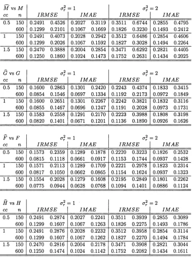
Each function was estim ated a t a 50 x 50 equally spaced grid in [0,1] x [0,1] when n = 150, and at another 60 x 60 uniform grid on the same dom ain when n = 600. Two criteria sum m arizing goodness of fit were calculated, the Integrated R oot Mean Squared Error (IRMSE) and Integrated Mean Absolute E rror (IM AE), a t all grid points and then they were averaged. Tables 2.1 and 2.2 report the m edian of these averages over 2000 replications for each design, scenario and bandw idth. They also report the results obtained when using the estim ators proposed by Linton and Nielsen (1995) when (2.5.1) is used, and Linton and Hardle (1996) when (2.5.2) is used instead, on the first column from the left under each fitting criteria respectively. They were constructed using the same unrestricted first stage nonparam etric regression used by our estim ator.

2.5 Num erical Results

F relative to estim ates of G. There does not seem to be a dram atic difference in estim ates of H between estim ators in b o th designs. All sets of estim ates deteriorate when a r is increased.

Unknown Link Function

As it was pointed our earlier, when d = 1, model (2.1.1) is nested in th e class of models Horowitz (2001) considers. Consequently, it is n a tu ra l to make a comparison with his estim ator in this specific case. We replicated Horowitz (2001) original experim ent1 which is as follows: 1000 observations (Y, X, Z) were generated from, Y = 1 (G ( X ) + F (Z) — e > 0), where e ~ N (0,1), X ~ N (0,16) and Z ~ N (0,16), and independent of each other. The functions G, F and H are2

G (x) = 3 sin ^ x ,

F (z) = 3 [exp (0.35,z) — 1], and H (m) = $ ( m ) ,

where $ is the standard normal distribution function. This is a binary probit model, where P r ( y = l \ X = x, Z = z) = $ (G (x) + F (z)) = r (x, z).

Horowitz (2001) (NP2) used the following fourth and second order kernels to estim ate G, F and H\

105

K (u) = — — ( l — 5u 2 + 7u 4 — 3 u6 ) 1 ( |u | < 1 ) ,

64

Kh ^ = i f ^ “ U 1 ^ '

T he weight functions used to calculate G, F and H were W2 (x) = K h { x ) , w\ (z) = (1/2) ( z /2), and w h ( x , z ) = W2 (x ) w \ (z) respectively. He also used bandw idths h \\ =

6, h,2\ = 5, and h n = 3.25. He chose these bandw idths through M onte Carlo experimen­

tatio n to approxim ately minimize the unweighted Integrated M ean Squared Errors of his estim ators of G, F and H . The additional bandw idths his estim ator needs were set using his suggested rule-of-thum b, 2 = h k \ n ~ l f7 2 for k —1,2.

We im plem ent our proposed estim ator (NP1) for this design, using a second order Gaus­ sian kernel as before, w ith p\ = 0, P2 = 1, and p* = 1. We also found th e optim al band­

w idths hi = 0.925, /12 = 2.5 and h* = 0.2 for this design, by M onte Carlo experim entation as Horowitz (2001) did.

1T he computer code we wrote to implement Horowitz (2001) estim ator, was not fast enough to conduct large scale sim ulations as before.

2.5 Numerical Results

Figure 2.1 shows the standardized Q - Q plots of b oth set of estim ators at different points well in the interior of the support of each function. These points were chosen sufficiently far from the boundary of the d a ta to avoid boundary effects for b o th estim ators. These plots were based on 300 replications. We observe th a t the norm al approxim ation of our estim ator for G and F are b e tte r th a n Horowitz’s at the chosen points. Similar results (not presented) hold for other points well in the interior of the support of (X , Z ) for G and F. On the other hand, th e norm al approxim ation of our estim ator for H is sim ilar to Horowitz’s for low values of m only, while it outperform s Horowitz’s for higher values.

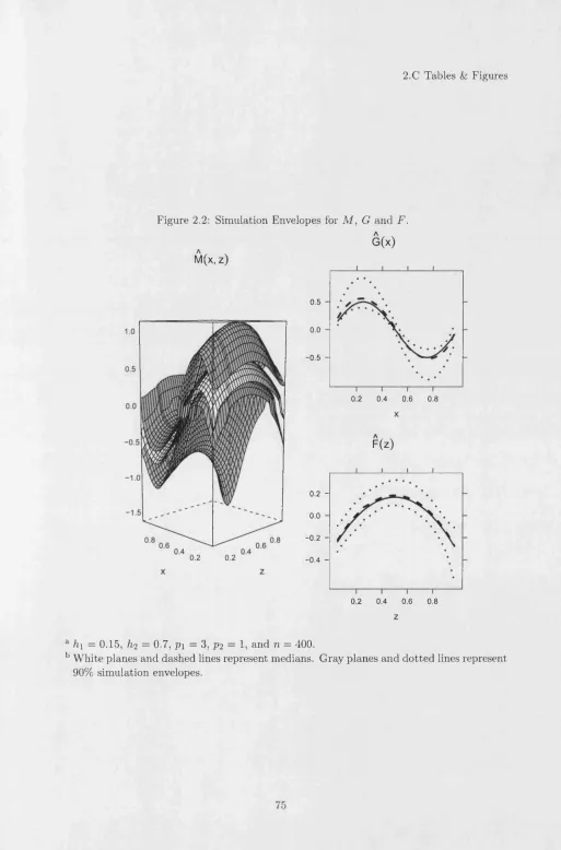
Finally, Figure 2.2 displays a visualization of th e resulting o u tp u t of 5000 replications of a fourth design using only our procedure. D ata was generated as before w ith the same G and F , b u t H [m] = 1 + (16/7) m, w ith o% = 1. O ther inform ation was set accordingly, for example n = 400, h\ = 0.15, /i2 = 0.7, p\ = 3, and P2 = 1. The white plane and

dashed lines represent m edians of simulations, and gray planes and dotted lines represent 90% sim ulation envelopes.

2.5.2

Generalized Homothetic Production Function Estimation

Let y be the log o u tp u t of a firm and (z, z) be a vector of inputs. S tarting w ith Shephard (1953) and Shephard (1970), many param etric production function models of the form y = r* (x, z) + £r * have been estim ated th a t impose either linear hom ogeneity or hom otheticity for the function r. In the homogenous case, corresponding to known H (m) = m, many models have been proposed, see Bairam (1994) and Chung (1994) for param etric examples, and Tripathi and Kim (2003) and T ripathi (1998) for fully nonparam etric options. Zellner and Ryu (1998) provides empirical comparisons of a large num ber of different hom othetic production functional forms. In the nonparam etric framework3, Lewbel and Linton (2006) presents an estim ator for a hom othetically separable function r*.

However, a more general definition of homogeneous and hom othetic functions is given below:

Definition 2.5.1

5Rd+1

>

zs

on ^w i f and only i f the equation M* (Aw) = g (A) M* (w) holds f or all (A, w) G 3£++ x ^w

such that Aw G Sfrw. The function g : 5?++ —» is such that g ( 1) = 1 and dg (A) / d \ > 0 for all A.

2.5 Numerical Results

D e fin itio n 2 .5 .2 A function r* : C —♦ 5? is said to be generalized homothetic on i f and only i f r* (w) = H [M * (iu)], where H : 3? —> 3? is a strictly monotonic function and M* is generalized homogeneous on tyw.

It is clear from Definitions 2.5.1 and 2.5.2, th a t hom ogeneity of degree k and homoth- eticity are the special case in which the function g takes the functional form g (A) = XK. Given a generalized hom othetic production function we have

r* (£, z) = H [M* (x, z)] = H \ m * {x/z,1) g (1 / z ) ~ l

= H [ G (x) F (z)\ = H [ M (x, z)\ = r {x, z ), (2.5.3) where x = x / z and F (z) = 1/g (1 f z) . W hen H is assumed known and equal to the identity function, T ripathi and Kim (2003) and Tripathi (1998) use th e assum ption th a t M [x,z) is a homogeneous function of degree one, i.e. F (z) = l / z , in order to identify the model and achieve dim ensionality reduction. Lewbel and Linton (2006) used the same functional assum ption regarding F b u t w ith an unknown strictly m onotonic link function H. In the contrary, the proposed estim ator in this chapter could easily be implem ented in order to identify M , G, F and H in models such as (2.5.3), i.e. y = r ( x , z ) + £r > w ithout imposing any such param etric specification of F, b u t exploiting the p artial separability of M with respect to z instead along with the fact th a t f (z) > 04. For the same reasons, it does also reduce the dim ensionality by 1 as explained earlier.

We have built an R package, JLLprod, which along w ith its m anual can be freely down­ loaded from the a u th o r’s website. After installation, the user also has access to a production d ata set from the Ecuadorian economy in 2002, and will be able to reproduce the informa­ tion presented in this section. We then use it in order to estim ate generalized hom othetic production functions for four industries in m ainland C hina5 in two tim e periods, 1995 and 2001. For each firm in every industry, we observe the net value of real fixed assets K, the num ber of employees L, and Y defined as the log of value-added real o u tp u t. K and Y are m easured in thousands of Yuan converted to the base year 2000 using a general price deflator for the Chinese economy. For details regarding the collection and construction of this d a ta set, see Jefferson, Hu, Guan, and Yu (2003).

We consider b o th nonparam etric and param etric estim ates of th e production function r ( k, L) G V, which is a set of sm ooth production functions, and k = K / L as in (2.5.3). To eliminate extrem e outliers in b oth sets of estim ates, we sort th e d a ta by k and remove the top and b o tto m 2.5% of observations in each industry and year. B oth regressors were also

4As d g (A) / d \ > 0, and A = z ~ x, it follows th at F (z) is strictly increasing, i.e. f (z) = d F ( z ) / d z > 0 over its entire domain.

2.5 Num erical Results

normalized by their respective m edian prior to regression.

Parametric

Consider a general production function (P I) in which log o u tp u t Y — r ^ pl (k, L) + er , where

r1j)pi (k, L) = 0O + 0i In (k ) + 02 In {L + 7) + 03 [In (fc)]2

+ 04 In (k) In (L + 7) 05 [In (L + 7)]^ , (2.5.4) and ^ p i = (0o, 0 i ,02,03,04, 0s)T - W hen 20105 — 0204 = 0 and 6\Q§ — 0^03 = 0, this general

model nests the following generalized hom othetic production function (P2) specification, M (k, L) = k a {L + 7)

r^ P2 (k, L) = H (M ) = /?o + f t In (M ) + f t [In (M)]2 , (2.5.5) where ipP 2 = (a , f t , /3i, f t ,7)T - Furtherm ore, if we also impose a th ird param eter restric­

tion6, 7 = 0, we obtain the hom othetic Translog production function (P3) of Christensen, Jorgenson, and Lau (1973) as a special case as well, i.e.

M ( k , L ) = k aL

7 ^ 3 (*, L) = H (M ) = f t + f t In (M ) + f t [In (M)]2 , (2.5.6) where ipP 3 = (a, f t , f t , f t ) T .

Figure 2.3 shows isoquants for P2 with ipP 2 = ( 1 /2 ,1 0 ,1 /2 ,1 ,7 ) T, where 7 = —1,0, +1.

At any level of o u tp u t, these isoquants are steeper at high levels of k for negative 7 th an for positive 7. However, as in the hom othetic case, 7 = 0, the slopes of their level surfaces are constant along rays through the origin. This im portant property is preserved by this more general specification.

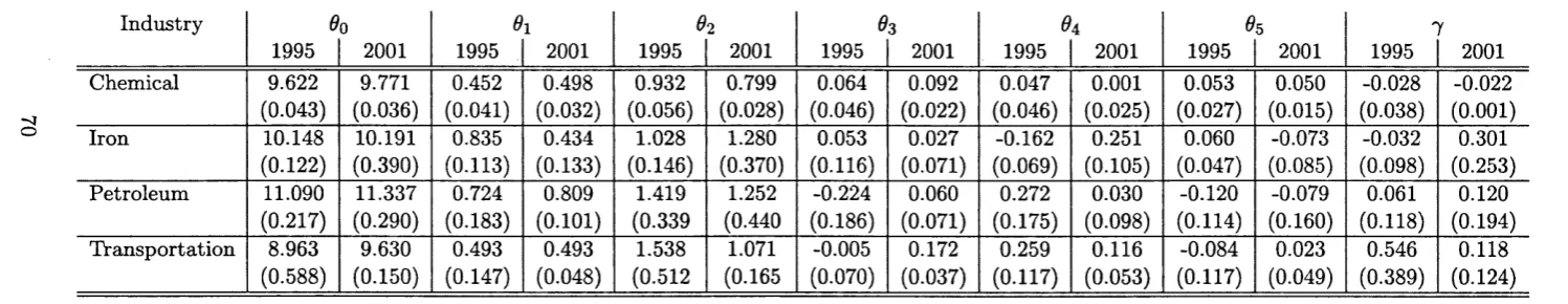
F ittin g these models by Nonlinear Least Squares in each year yields the param eter es­ tim ates reported in Tables 2.3-2.5 (Heteroskedasticity robust stan d ard errors are in paren­ theses).

2.5 Numerical Results

S p e c ific a tio n T e s t

Two sets of param etric restrictions are tested on model (2.5.4) for each year and industry. In order to assess w hether model (2.5.4) may be further simplified by (2.5.5),

Hq : 20105 — 02$4 = 0; $l e5 - e p3 = o

is tested by means of a Wald statistic, W n which is distributed under Ho as X(2) • A further

simplification, (2.5.6), is also tested by a Wald statistic, W13, which under the H0 : 20105 — = 0;

0105-0203 = 0; 7 = 0,

is distributed as %(3). The results of these tests are presented below.

Industry

w12

1< p-value

)95

W13 p-value W i2

2 0( p-value

)1

W13 p-value

Chemical 1.280 0.527 2.244 0.523 17.286 0.000 1,095 0.000

Iron 8.834 0.012 14.261 0.003 2.272 0.321 2.343 0.504

Petroleum 1.790 0.409 3.076 0.380 0.791 0.673 0.813 0.846

T ransportation 1.735 0.420 1.997 0.573 7.980 0.019 8.252 0.041

Models (2.5.5) and (2.5.6) are valid param etric simplifications of the general production function (2.5.4), except for the iron industry in 1995 and the chemical and transportation industries in 2 0 0 1.

T he suitability of the param etric Generalized H om othetic and Translog production func­ tion fits, r^ 2 (k , L) and in these industries may be also judged by the use of a residual based test. For this purpose, we decide to employ th e test proposed by Zheng (1996) for the hypothesis

Ho : r e V { r E V \ r = r ^ pi for some ippi} . For I = 2,3, their te st statistics are given by

1 n n

U”

= 12^2 E £ (y‘ - (*.

LJ) (Y> - rf Pl

Li)) K

i=l j=l

2.5 Numerical Results

w ith kernel K (•), the Gaussian kernel here, and bandw idth A, set equal to hi in all cases. Given some regularity conditions, under the null hypothesis th a t the param etric specifica­ tions are correct,

nXUpi ~ N ^0 ,2

J

J

by replacing integrals by sums and unknown functions by their nonparam etric estim ates in (2.5.7) and (2.5.8), we obtain the following test results:

Industry

A

1995

Up2 p-value A

2001

UP 2 p-value

Chemical 5.125 -0.7698 0.7793 2.25 -0.4728 0.6818

Iron 4.250 -0.7532 0.7743 4 -0.7367 0.7693

Petroleum 2.750 -0.8117 0.7915 11 -0.7325 0.7681

T ransportation 1.750 -0.6519 0.7428 4.37 -0.7124 0.7619

A UP 3 p-value A UP 3 p-value

Chemical 5.125 -0.7721 0.7800 2.25 -0.4130 0.6602

Iron 4.250 -0.7195 0.7641 4 -0.7417 0.7709

Petroleum 2.750 -0.8088 0.7907 11 -0.7327 0.7681

T ransportation 1.750 -0.6503 0.7422 4.37 -0.7065 0.7601

We fail to reject b oth Ho for all industries in b oth years at any level of significance. In all cases, test results are not altered by the choice of smoothing param eter A. B oth sets of results justify the use of b oth models as sensible param etric simplifications of th e d a ta7 against which we may compare our more flexible specification. O ther kernel-based specification tests are Bierens (1990), Hardle and M ammen (1993), Gozalo (1993) and Horowitz and Spokoiny (2001), for example.

N o n p a r a m e tr i c

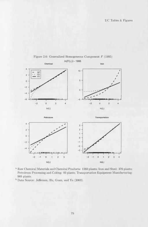
Figures 2.4 to 2.11 show generalized hom othetic nonparam etric estim ates M (fc,L ), G ( k ) , F (L) and H (M ) for b o th years. For each industry and year, we use local quadratic regres­ sion w ith a Gaussian kernel and bandw idths, h\, given by a stan d ard unrestricted leave-one- out cross validation m ethod for regression functions. In the second stage, we set bandw idth h-2 to be the same in local linear regressions across industries and tim e. We also choose the

2.5 Num erical Results

location and scale norm alizations through experim entation to o btain estim ated surfaces M with approxim ately the same range, yielding the following norm alizations:

Industry

n

1995

In Lq _ro n

2001 In L0 ro

Chemical 1560 3.40 7 1637 3.06 7.0

Iron 376 -0 .3 7 7 341 4.06 8.0

Petroleum 93 2.73 7 119 2.27 8.5

T ransportation 989 3.44 7 1230 4.04 7.5

The nonparam etric fits of the generalized homogeneous com ponent, M , shown in Figures 2.4 and 2.8, are quite similar. They are b oth increasing in k and L w ith ranges varying more with labor th a n w ith respect to capital to labor ratios, as we would expect8. N onparam etric estim ates of th e functions G and F are different to the param etric Translog model estim ates (P3) in Figures 2.5, 2.6, 2.9 and 2.109, b u t they are roughly sim ilar to param etric generalized hom othetic model (P2) a t low levels of L. They are all strictly increasing in their argum ents, but show quite a bit more curvature, departing most m arkedly from the param etric models for F in 1995 and G in 2001 for most industries. Com paring the nonparam etric estim ator of F , in Figures 2.6 and 2.10 , with the param etric ones also provides a quick reference to