Geographic Routing with Logical Levels forwarding
for Wireless Sensor Network
Yassine SABRI
STIC Laboratory
Chouaib Doukkali University, B.P: 20 El Jadida MOROCCO
Najib EL KAMOUN
STIC Laboratory
Chouaib Doukkali University, B.P: 20 El Jadida MOROCCO
ABSTRACT
Location information is essential in many applications of WSNs,it is natural to use this information for routing as well. Location-based protocols or geographical routing protocols to exploit the location information of each node to provide efficient and scalable routing. Various routing algorithms that feat geographic information (e.g., GPSR) have been aimed to attain this goal. These algorithms re-fer to all nodes by their location, not address, and use those coor-dinates to route greedily, when possible, towards the destination. However, there are dozen’s situations where location information is not available at the node. This paper presents a new geographi-cal routing protocol for Wireless Sensor Networks (WSN) energy-efficient data forwarding, called GRPW(geographic routing proto-col washbasin).Protoproto-col GRPW ensures a load balancing, minimiz-ing energy consumption and the rate of message delivery usminimiz-ing a routing policy with logical levels, inspired from the water flow in a washbasin, without making the assumption that all sensors are localized. GRPW protocol performance compared to the tocol GPSR show that maximizes the lifetime of the network, pro-vides quality service parameterizable, and is appropriate for dense sensor networks confronting our method to an optimal algorithm.
General Terms:
Routing, wireless sensor network (WSN)
Keywords:
Wireless Sensor Network (WSN), Geographical Routing ,Local-ization.
1. INTRODUCTION
Wireless Sensor Networks (WSN) are constituted of a large number of tiny sensor nodes randomly distributed over a geographical region whose power consumption is low. How-ever, as shown in current research [11] , the classical routing protocols are not applicable to sensor networks in a real en-vironment,mainly because of specific radio conditions.Noise, interference, collisions and the volatility of the node neigh-borhood leading to a significant drop in performance. Many applications for sensor networks such as monitoring of forest fires, the remote meter reading,...For these cases,The Geo-graphic routing of data in this type of network is an important challenge,Geographic routing uses nodes’ locations as their addresses, and forwards packets (when possible) in a greedy manner towards the destination. The most widely known proposal is [5][8], but several other geographic routing schemes have been proposed [14] One of the key challenges in geo-graphic routing is how to deal with dead-ends, where greedy
routing fails because a node has no neighbor closer to the destination; a variety of methods (such as perimeter routing in GPSR/GFG) have been proposed for this. More recently, GOAFR [10] proposes a method for routing approximately the voids that is some asymptotically worst case optimal as well as average case efficient. Geographic routing is scalable, as nodes exclusively maintain state for their neighbors, and supports a full general any-to-any communication pattern without explicit route establishment. However, geographic routing requires that nodes know their location. While this is a natural assumption in some settings (e.g., sensornet nodes with GPS devices), there are many circumstances where such position information isn’t available.are most often require information about the position of their voisins to function effectively.Or, this assumption is far from the reality.The other, the localization of protocols, used as a preliminary step by geographical routing protocol are not necessarily precise. For example, in [15],the authors proposed localization methods with which sensors determine their positions with a rate of less than about 90% positioning in large scale. or, if a node that does not know its location, the node risk of never communicate with other node of networks,and no information will be transmitted to the user and the base station never knows that node.
In this paper, we propose a geographic routing protocol which is based on the construction of a logical topology levels. This strategy allows the construction the incline level directed to the sink node. To make the sensor network similar to a washbasin and routing the packet to the flow of water in this washbasin. We assume that among the node deployed that there are well-positioned nodes and other non-positioned. Our work is decomposed into two phases: Phase 1: one starts by constructing a logical topology by forming the logic levels , each level is char-acterized by a width that depends on the network density, Then for each node will be well localized we assigned to it a level depending on the distance which separates him to the node sinks. subsequently the non-localized nodes will join the level closest according to neighborhood nodes by sending specific messages, at the end of this phase each node must have a level of belonging.
Phase 2: This phase consists of a transmit data to sink node,data transmission is performed in three modes of progression: the first mode to route the packet to a neighbor who belongs to a higher level,however, if they find no neighbor in the level above it switches to Second mode to transmit the packet to a neighbor who belongs to the same level,otherwise the packet will deliver-ing to third mode in case there are some holes must reroute the packet to the lower level.
present our new localization algorithm GRPW. In Section 5, we evaluate the proposed scheme through comprehensive simulation studies and compare it with GPSR technique. We conclude the paper in Section 6.
2. RELATED WORK AND BACKGROUND
With the development of wireless ad hoc networks like roofnets [17][18] and sensornets [7][12], there has been a proliferation of geographic routing algorithms in recent years .
The geographical routing emphasizes the fact that each node in knows its coordinates geographical and uses those to the final destination for routing decisions. Early work in geographic routing considered only greedy forwarding [16] by using the locations of nodes to move the packet closer to the destination at each hop. Greedy forwarding fails when reaching a local maximum, a node that has no neighbor closer to the destination. CompassII [9] presents a face routing algorithm that guarantees message delivery on a geometric graph by traversing the edges of planar faces intersecting the line between the source and the destination. [5] discuss algorithms for extracting planar graphs from unit graphs and for face routing in the planar graphs to guarantee delivery. Due to the inefficient paths resulting from face routing, they propose combining face routing with greedy forwarding to improve the path length.
GPSR protocol [8] is the earliest geographical routing protocols for adhoc networks which can as well be applied for WSN surroundings. The GPSR adapts a greedy forwarding strategy and perimeter forwarding strategy to route messages. It makes uses of a neighborhood beacon that sends a node’s identity and its position.Each packet contains the position of the des-tination and nodes necessitate only local selective information concerning their emplacement and their immediate neighbors’ positions to forward the packet. Each node forwards the packet to the neighboring nodes nearest to the destination using greedy forwarding.When greedy forwarding fails, face routing is employed to route roughly dead-ends until closer nodes to the destination are found.
Recently, there have been proposals [13][14] for geographic routing without location information. The approach is to assign logical coordinates to each node and then apply greedy forward-ing over the logical coordinates.To route from u to v with GEM primitive routing algorithm, a message is delivered following a node’s parents until a parent’s virtual angle contains v’s virtual angle. Then the message is delivered through every child that comprises v’s virtual angle until v. In order to build the logical space, a relatively large establish overhead is necessitated in the form of various global floods or iterations of coordinates’ relaxation. Extra overhead is incurred to detect and propagate changes in the logical coordinates due to topology changes. Although it has some benefits, GEM is not as efficient and scalable as routing with location information. Perimeter routing as well cannot be used in these strategies, and in [14] there is no solution provided for dead-ends that guarantees delivery. In addition, for data-centric memory, these schemes do not allow for robust reproduction and consistency.
Another problem problem of geographic routing is that packets may be routed to a dead end. The distance from a sensor to the base station is marked alongside the sensor. Suppose there is no sensor to the right of the dashed line, which outlines an open void. The void may be a disaster area where all sensors are destroyed, or it may be a bay where the sensors cannot survive. There is a single dead end, which does not have any neighbor that is closer to the base station. Once a packet is routed to the dead end, it cannot proceed any further. The packets from the gray nodes will be forwarded to the dead end based on geographic routing.To solve the above problem, GPSR use the "right-hand rule" to route packets along the boundary of the void
until they reach the other side of the void. This approach finds a specific detour path out of the dead end.
In this paper we address how to keep back the gains of ge-ographic routing in the absence of localization information. This problem has been partially addressed in [6], but there they consider the case where some nodes don’t have geographical data; here we focus mainly on the case where no (or only the perimeter) nodes have location information. Our approach involves assigning virtual logical levels to each node and then applying standard geographic routing over these levels of belonging. These levels virtual need not be precise represen-tations of the inherent geography but, in order to serve as a basis of routing, they must reflect the underlying connectivity. Thus, we construct these virtual coordinates using mainly local connectivity information and the destination position sink. Since local connectivity information is ever available (nodes perpetually know their neighbors), this technique can be applied in most settings. Moreover, as our simulation consequences demonstrate, there are scenarios, such as in the presence of obstacles, where greedy routing performs better using virtual logical levels than using true geographic coordinates.
3. MODEL
First we describe the system model on which our protocol design is based. In this paper ,we focuse on static networks. Moreover, it assumes that all sensors have identical reachability radiusr. However, it is easy to adapt our method to sensors having different reachability radius. A wireless sensor networks is represented as a bidirectional graphG(V, E)whereV is the set ofnnodes representing sensors andEis the set ofmedges representing communication links. If two nodesu, v ∈ V are neighbors, then they are linked that means distance betweenu
andvis smaller thanr. The set of neighbors for a nodeu∈V
is noted N(u). The nodes have knowledge of their location through some other means, such as GPS or simply explicit programming. The set of nodes is notedΛ. The set of neighbor anchors for a nodeuis notedNΛ(u)(NΛ(u) =N(u)∩Λ)and the set of non-neighbor nodes that know their position is noted
NΛ(u)(NΛ(u) = Λ/NΛ(u)). Note that all identical nodes (anchors or others nodes) have the same capabilities (energy, processing, communication, ...). The coordinate of a position of nodeuis noted(xu, yu).Pis the set of all possible positions in a network.
4. GEOGRAPHIC ROUTING PROTOCOL
WASHBASIN
We assume in this work that each node can get its own location information either by GPS or other location services [19][15]. Each node can get its one-hop neighbor list and their locations by beacon messages. We consider the topologies where the wireless sensor nodes are roughly in a plane.
Our approach involves three steps:
(1) The distribution of the sink address to the set of sensors networks:In the first step,The communications in this step are made in three steps:
—When a node wants to transmit the sink position to its neighbors ,it first emits ADV message containing the lo-cation of sink.
—A node receiving a message ADV. If interested in this in-formation, it sends a message REQ to its neighbor. —In Receiving a message REQ, the transmitter transmitted
(2) Construction of logical levels: In this step the node networks determine its level of belonging through the sink node position,each nodeuwell localized, calculate its level based on the received position of sink in thePhase 1,with whichucalculates the distanceduSinkwhich separates him with the sink node .the levels is calculated so that the width levelηbe constant is less than and inversely proportional to the density of networksδ.
The levellof the nodeudefined by:
Levelu={l∈N/duSink
η ≤l≤ duSink
η + 1}
Set of the neighbor nodes that are well localized and which belongs to the same level asu:
LNΛ(u)={v∈NΛ(u)/Levelu=Levelv}
Set of the neighbor nodes that are well localized and which belongs to the higher level thanu:
L+N
Λ(u)={v∈NΛ(u)/Levelu=Levelv−1}
Set of the neighbor nodes that are well localized and which belongs to the lower level thanu:
L−N
Λ(u)={v∈NΛ(u)/Levelu−1 =Levelv}
For non-localized node, they determined their level of belonging by sending a message belonging to neighboring nodes, the neighboring node that received the message, reply with a message containing its level of belonging, the level ofuis equal to the level of maximum neighbors that they like the nivau.
A B C
D E
F
G
H
I
J K
L M
N
O
P Q R
S
T U
V W Z A1
B1 C1
D1 E1
F1
G1 H1
I1 J1 K1
L1 M1
N1 O1
P1
Q1
[image:3.595.57.283.485.712.2]R1 S1
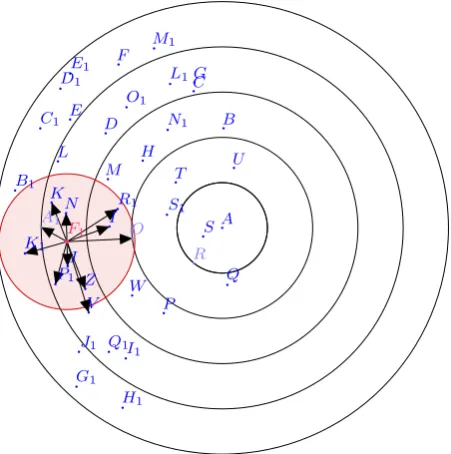
Fig. 1. The calculated level for a not localized node
Figure 1 shows an example of a sensorF1not localized who is seeking to determine its level of belonging, the node begin
scanning its neighbor by sending aHELLOmessage, to cal-culate the number of node of each level{2,3,4},F1ranking neighbor as followingL−N
Λ(F1) = {A1, K1},L + NΛ(F1) =
{R1, O, I}andLNΛ(F1) ={P1, K, N, Z, V}. like that he decided to join the level3ofLNΛ(F1)that has the maximum number of nodes.
(3) Data forwarding :the routing decision is done in our ap-proach in three modes (Figure 5 shows the pseudo code of GRPW)., depending on dispoinibilites neighboring nodes and of their level of belonging: theEven Forwarding, An-terior Forwardingand theRear Forwarding (respectively called EF, AF and RF).
—The AF constructs a road traversing the nodes of the source to the destination which each node receiv-ing a packet DataPacket with the mode of transport
ANTERIOR_FORWORD, will move toward the intermediate
node in its coverage area and belongs to the level 1 , the intermediate node select among the neighboring node which belongs to the levels using a lookup function. Lookup function is used by a node in order that he can de-termine the next hop to reach the next level, to dede-termine the next hop function, lookup based on the principle of Round Robin (RR), Round-robin (RR) is one of the sim-plest scheduling algorithms for processes in an operating system. As the term is generally used, time slices are as-signed to each process in equal portions and in circular order, handling all processes without priority (also known as cyclic executive),Using RR will enable us to balance the traffic on all node resaux and exploit several paths for routing the packet. The routing metric which we define is composed of the residual energy and node density. The figure 2 is an example of theAnterior Forwardrouting technique represent by the segment in green color ,the sensor Z belongs to levelLevelZ= 3seeks the next hop neighbor among the setL+N
Λ(Z)={I, W}of neighbors belonging to level4, Z selects I as next hop based on the lookup function.
A B C
D E
F
G
H
I
J K
L M
N
P Q S
T U
V W Z B1
C1 D1E1
F1
G1 H1
I1 J1 K1
L1 M1
N1 O1
P1
Q1
R1 S1
q
Fig. 2. Anterior Forward for the node Z
[image:3.595.320.543.488.697.2]change the routing mode toEVEN_FORWORDmode to reroute the packet in EF Mode. u will also delegate the responsibility to transmit the packet he received to the nearest neighbor node sink that he has the same level as u. This process is repeated recursively until reaching a node that can move the packet to the nodes of levelL+N
Λ().
—Because of the frequent failures of nodes, node mobil-ity or policy scheduling of activities used, disconnec-tions can occur in the network generates, well, what are called "Voids". In this situation,we switching to the EF mode.The EF consists of finding a path for a packet that did not find a next hop neighbor in levelL+N
Λ() using the AF mode, EF is defined as follows: When a packet DataPacket, arrives at a node x from node y, the way forward is the next one is at the same level of belong-ingLNΛ()while avoiding the "crossing links" (route al-ready traveled), this is why each packet keeps his foot-steps (noued list, crossing EF in Mode or RF) in the vector
DataPacket: IntermediateNodesthe next hop is
se-lected by the lookup function that returns a noued neigh-bor who belong to the same level as x and that do not belongs to all the nodes already traversedDataPacket:
IntermediateNodesto of avoids the routing loop
A B C D E F G H J K L M N P Q S T U V Z B1 C1 D1E1 F1 G1 H1 I1 J1 K1 L1 M1 N1 O1 P1 R1 S1 l c1
Fig. 3. Even Forwarding for the node Z
The figure 3 is an example of theEven Forwarding rout-ing technique represented by the red segment,the sensor Z belongs to the levelLevelZ = 3, Z seeks the next hop neighbor among the set of neighbors belonging to the level 4 but when there is no node that belongs to levelL+N
Λ(Z) , Z will route the packet to the neighbor nodes of the same level as Z by selecting from the set
LNΛ(Z) = {V, N, P}based on the lookup function, Z will rerouting the packet to the node N.
—RF consists of reroute a packet DataPacket, who was failed in AF and EF, RF fact sends a packet to the low levelL−N
Λ()by seeking the next hop among neigh-boring based on the lookup function. RF is leaning on same technique used in Ef, for avoids the rout-ing loop we safeguard the sets of node traversed by the packet DataPacket in a vector-type structure
DataPacket:IntermediateNodes. The figure 4 is an
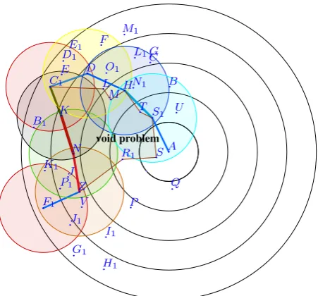
example of theRear Forwarding routing technique rep-resented by the green segment,the sensor C belongs to the
[image:4.595.315.541.96.306.2]void problem A B C D E F G H J K L M N P Q S T U V Z B1 C1 D1E1 F1 G1 H1 I1 J1 K1 L1 M1 N1 O1 P1 R1 S1
Fig. 4. Rear Forwarding Forwarding for the node K
Algorithm 4.1:When a node n receives a message data (DataPacket)
if(DataPacket.ModeForward=ANTERIOR_FORWORD) then
Neighbor=Lookup(DataPacket,TableLevel+1) ifNeighbor6=NULL
then
DataPacket.IntermediateNodes.Clear() Forward(DataPacket,Neighbor)
else
DataPacket.ModeForward←EVEN_FORWORD
GRPW(DataPacket)
else if(DataPacket.ModeForward=EVEN_FORWORD)
then
Neighbor=Lookup(DataPacket,TableLevel+0)
ifNeighbor6=NULLandNeighbor∈/DataPacket.IntermediateNodes
then
(DataPacket.IntermediateNodes.add(CurrentNode)
DataPacket.ModeForward←ANTERIOR_FORWORD
Forward(DataPacket,Neighbor) else
DataPacket.ModeForward←REAR_FORWORD
GRPW(DataPacket)
else if(DataPacket.ModeForward=REAR_FORWORD)
then
Neighbor=Lookup(DataPacket,TableLevel−1)
ifNeighbor6=NULLandNeighbor∈/DataPacket.IntermediateNodes
then
(DataPacket.IntermediateNodes.add(CurrentNode)
DataPacket.ModeForward←ANTERIOR_FORWORD
[image:4.595.57.281.348.556.2]Forward(DataPacket,Neighbor) else{DELET(DataPacket)
Fig. 5. Description of GRPW algorithm
levelLevelK = 3, k seeks the next hop neighbor among the set of neighbors belonging to the level 4 but when there is no node that belongs toL+N
Λ(Z) or same level as C which belongs toLNΛ(K)(the sensor C will be ex-cluded because it belongs to the nodes already traversed defined byDataPacket.IntermediateNodes) , K will route the packet to the neighbor nodes of the low level as K by selecting from the setL−N
Λ(K)={C, B, E}based on the lookup function, Z will rerouting the packet to the node B.
The finite state machine shown in Figure 6 depicts var-ious states which summarizes the three routing mode in the protocol GRPW ,depending on existence of neighbors node of each logical levels.
5. SIMULATIONS AND RESULTS
ANTERIOR_FORWORD MODE
EVEN_FORWORD MODE
REAR_FORWORD MODE Recepction ofDataPacket
Destroying the packet N oN eighbor /∈L+
NΛ() N eighbor∈L+N
Λ()
N oN eighbor /∈L0
NΛ()
N eighbor∈L+
NΛ()
DataPacket.ModeForward=ANTERIOR_FORWORD
DataPacket.ModeForward=EVEN_FORWORD
DataPacket.ModeForward=REAR_FORWORD
N oN eighbor /∈ {L0
NΛ(), L
− NΛ(), L
+
[image:5.595.57.266.110.240.2]NΛ()}
Fig. 6. Finite state machine of GRPW protocol
use of unidirectional antennas) is simulated in J-Sim. Therefore, the vicinity of a node in terms of transmission range is not nec-essarily spherical.Note that there several simulators in the liter-ature such as GlomoSim[3], OMNET++[4], OPNET[2], NS-2[1]. The MAC layer is considered perfect and the transmission of messages are without loss in our simulation.
To study and analyze the performance of the protocol, three met-rics are chosen: (i) average dissipated energy in sensor nodes, (ii) delivery rate,(iii) energy consumption . Average dissipated energy is the ratio of total energy dissipated in the network to the number of packets received by the sink over a given period of time. The performance of the proposed protocol is studied with respect to the above three metrics with varying network sizes. Each simulation is carried out with 10 different topologies and the final results are presented based on the average of the result sets.
The node density in the network is increased from 5 to 14 with 3 being added in every step of increment. Initially, the sen-sors nodes are randomly distributed on a200m×200marea (A= 200×200),the radio range for each sensor is kept at 15m. Firstly,to learn how to we must select the width of logic levels
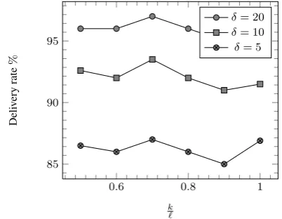
η, we begin by analyzing the Impact of network densityδand width on the rate of packet delivery. as cited in, for routing and forwarding the data in Gwap operates through logical levels re-quires that the width for each level be inversely proportional to the density of networks, which it interprets as
η=k
δ (1)
through other, for a node can communicate with the level nodes must its transmission rangeris less than the widthη:
η≤r≤2η⇒0.5×r≤η≤r (2)
The density of a sensor networkδis the average number from neighbors for a node. It is obtained by the following equation:
δ=n×π×r 2
A (3)
which implies that:
r= r
A×δ
n×π (4)
According to (1) and (2):
0.5×r≤ k
δ ≤r (5)
we replacingrby its value:
0.5×
r
A×δ
n×π×δ≤k≤
r
A×δ
n×π ×δ (6)
placing:
`= r
A×δ
n×π×δ (7)
which implies that:
0.5×`≤k≤` (8)
The graph show the impact ofk on the performance of gwt in terms of delivery rate,it is clear that the best value isk= 0.7×`, it is the value that will be used later.
0.6 0.8 1
85 90 95
k `
Deli
v
ery
rate
%
[image:5.595.328.529.210.366.2]δ= 20 δ= 10 δ= 5
Fig. 7. density of sensor localized with Network densityδ= 14
5.1 Energy consumption
For each topology,we measured different parameters: the distri-bution of the remaining energy (average figure, and variance in) distribution of the remaining energy by partitioning the network into logic levels . (in figure )
5 8 11 14
80 85 90
A
v
erage
ener
gy
of
netw
ork
(%)
[image:5.595.323.536.482.663.2]GPSR GRPW
Fig. 8. Average remaining energy in different Densityδ
5 8 11 14 40
60 80 100
V
ariation
of
the
ener
gy
(%)
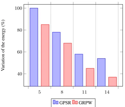
[image:6.595.65.277.94.275.2]GPSR GRPW
Fig. 9. Distribution of the remaining energy in different Densityδ
better distributed over the network with GRPW than GPSR, and this is because in the case of the Protocol GRPW, many nodes that are not localized are used to enable efficient routing.
200 400 600
80 90 100
Field width network (meters)
A
v
erage
Ener
gy
%
[image:6.595.64.276.358.527.2]GP SR GRP W
Fig. 10. Distribution of the remaining energy with network density δ= 14
200 400 600
60 70 80
Field width network (meters)
A
v
erage
Ener
gy
%
[image:6.595.321.534.427.594.2]GP SR GRP W
Fig. 11. Distribution of the remaining energy with network density δ= 5
5.1.2 The distribution of the remaining energy in large-scale. Figure 10 and Figure 11 show the average of the remaining energy on the network partitioned on virtual logical levels.We may remark easily that the energy is uniformly distributed within the network protocol with GRPW, compared to GPSR protocol. The advantage of such functionality for a routing algorithm is that it preserves the partitioning of a network into multiple sub-nets completely disconnected if there are nodes that fail or non-localized nodes in the case of GPSR protocol. In this case, no path end-to-end is available.
5.2 Delivery rate and transmission time
The graphs represented in figure 12 show the impact of of percentage of non-localized.In high density of localized nodes, whatever value of the delivery rate is close to100%. In low den-sity of localized nodes GRPW outperforms to GPRS. Through the use of several not localize node to route packets, the transmis-sion delay, end-to-end is significantly reduced by using GRPW. The packet loss rate as a function of percentage of non-localized nodes was also decreased as shown in Figure 12. These improve-ments in the delivery of packets can be explained by:
—percentage of nodes not used by GPSR, especially non-localized node.
—The use of a single path to forward packets to pout all flow will generate a long stay in queues leading to traffic congestion. —Packets can be lost due to severe resource constraints (buffer
size is very limited).
These results clearly demonstrate the ability of GRPW to issue binding flows and improve the quality of service compared to the protocol GPSR.
40 60 80 100
40 60 80 100
sensor localized%
Deli
v
ery
rate
%
GRPW GPSR
Fig. 12. density of sensor localized with Network densityδ= 14
6. IMPACT OF VOID SIZE
[image:6.595.65.277.584.753.2]50 100 150 200 250 300 70
80 90 100
The void radius (m)
Deli
v
ery
rate
%
[image:7.595.62.274.95.260.2]GRPW GPSR
Fig. 13. Delivery rate(%)depending on the size of the void
50 100 150 200 250 300
1 2 3
·10−2
The void radius (m)
Rate
of
control
pack
ets
%
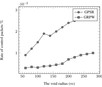
GPSR GRPW
Fig. 14. Rate of control packets(%)depending on the size of the void
hello messages and the hellobelonging messages which are sent periodically and are independent of topological changes. While in GPSR, the control messages used for route discovery and route maintenance are sent frequently due to the rapidly chang-ing topology of the network. Although GRPW uses only ?hello? and ’hellobelonging ’ messages as control messages, it shows higher routing overhead than GPSR. This is because GRPW does not need as many hello messages sent as GPSR to maintain its neighbouring table and its routing logical levels.
7. CONCLUSION
In this paper we present an algorithm called GRPW for assign-ing coordinates to nodes usassign-ing the logical levels in a wireless network (to be used for geographic routing) that does not require nodes to know their location. Our key contribution is a relax-ation algorithm that associates virtual logical levels to each node. These virtual logical levels are then used to perform geographic routing. Simulation results show that the success rate of greedy routing with virtual coordinates is exceedingly close to the suc-cess rate of greedy routing using true coordinates. Furthermore, in some cases such as in the presence of obstacles, greedy rout-ing with virtual logical levels significantly outperforms greedy routing with true coordinates. Intuitively, this is because virtual coordinates reflect the network connectivity rather of the nodes’ true locations which are less relevant in the presence of obstruc-tions.
We plan to extend this work in four directions. First, we intend to
continue the study of our algorithm by simulation using more re-alistic link layer models and network topology. Finally, we plan to implement our algorithm on sensor motes, and study it in real scenarios.
8. REFERENCES
[1] The network simulator. http://www.isi.edu/nsnam/ ns/, cited July 2010.
[2] Opnet technologies.http://www.opnet.com/, cited July 2010.
[3] About glomosim. http://pcl.cs.ucla.edu/
projects/glomosim/, cited July 2011.
[4] Omnet++ community site.http://www.omnetpp.org/, cited July 2011.
[5] Prosenjit Bose, Pat Morin, Ivan Stojmenovic’, and Jorge Urrutia. Routing with guaranteed delivery in ad hoc wire-less networks. InWIRELESS NETWORKS, pages 609–616, 2001.
[6] D. S. J. De Couto and R. Morris. Location proxies and in-termediate node forwarding for practical geographic for-warding. InProc. 4th Annual ACM/IEEE Intl. Conf. on Mo-bile Computing and Networking (MobiCom ’98), Dallas, TX, 1998.
[7] J. M. Kahn, R. H. Katz, and K. S. J. Pister. Next cen-tury challenges: mobile networking for smart dust. In Pro-ceedings of the 5th annual ACMIEEE international confer-ence on Mobile computing and networking, MobiCom ’99, pages 271–278, New York, NY, USA, 1999. ACM. [8] Brad Karp and H. T. Kung. GPSR: greedy perimeter
state-less routing for wirestate-less networks. InProceedings of the 6th annual international conference on Mobile computing and networking, MobiCom ’00, pages 243–254, New York, NY, USA, 2000. ACM.
[9] Evangelos Kranakis, Harvinder Singh, and Jorge Urrutia. Compass Routing on Geometric Networks. InProc. 11 th Canadian Conference on Computational Geometry, pages 51–54, Vancouver, August 1999.
[10] Fabian Kuhn, Rogert Wattenhofer, Yan Zhang, and Aaron Zollinger. Geometric ad-hoc routing: of theory and prac-tice. InProceedings of the twenty-second annual sympo-sium on Principles of distributed computing, PODC ’03, pages 63–72, New York, NY, USA, 2003. ACM.
[11] P. Levis, A. Tavakoli, and S. Dawson-Haggerty. Overview of Existing Routing Protocols for Low Power and Lossy Networks. IETF, Internet-Draft draft-ietf-roll-protocols-survey-07, April 2009.
[12] Jinyang Li, John Jannotti, Douglas S. J. De Couto, David R. Karger, and Robert Morris. A scalable location service for geographic ad hoc routing. InProceedings of the 6th an-nual international conference on Mobile computing and networking, MobiCom ’00, pages 120–130, New York, NY, USA, 2000. ACM.
[13] James Newsome and Dawn Song. Gem: Graph embed-ding for routing and data-centric storage in sensor networks without geographic information. InProceedings of the 1st international conference on Embedded networked sensor systems, SenSys ’03, pages 76–88, New York, NY, USA, 2003. ACM.
[image:7.595.63.274.293.473.2][15] Clément Saad, Abderrahim Benslimane, and Jean-Claude König. AT-Dist: A Distributed Method for Localization with High Accuracy in Sensor Networks. International journal Studia Informatica Universalis, Special Issue on "Wireless Ad Hoc and Sensor Networks", 6(1):N/A, 2008. [16] Ben L. Sayan, Ben Leong, Sayan Mitra, and Barbara
Liskov. Path Vector Face Routing: Geographic Routing with Local Face Information. InProceedings of the 13th IEEE International Conference on Network Protocols, ICNP ’05, pages 147–158, 2005.
[17] Timothy J. Shepard. A channel access scheme for large dense packet radio networks.SIGCOMM Comput.
Com-mun. Rev., 26(4):219–230, August 1996.
[18] Timothy J. Shepard. A channel access scheme for large dense packet radio networks. InConference proceedings on Applications, technologies, architectures, and protocols for computer communications, SIGCOMM ’96, pages 219– 230, New York, NY, USA, 1996. ACM.