The Decomposition of Inter Group Differences in a Logit Model: Extending the Oaxaca Blinder Approach with an Application to School Enrolment in India

Munich Personal RePEc Archive

The Decomposition of Inter-Group

Differences in a Logit Model: Extending

the Oaxaca-Blinder Approach with an

Application to School Enrolment in India

Borooah, Vani and Iyer, Sriya

University of Ulster, University of Cambridge

2005

The Decomposition of Inter-Group Differences in a Logit

Model: Extending the Oaxaca-Blinder Approach with an

Application to School Enrolment in India

Vani K. Borooah*

University of Ulster, Northern Ireland

Sriya Iyer#

University of Cambridge, England

June 2003

Abstract

This paper suggests a method of decomposing differences in inter-group probabilities from a logit model and shows how it can be related to similar decompositions derived from a Oaxaca-Blinder framework. In so doing, it offers a solution to a problem, embedded within the Oaxaca-Blinder decomposition, relating to the appropriate choice of common coefficient vectors with which to evaluate the different attribute vectors. The decomposition method also shows how pairwise comparisons of groups might be conducted in the presence of more than two groups, without discarding the information on groups excluded from the comparison. The proposed method is applied to inter-group differences in schooling participation in India and the results are compared with the Oaxaca-Blinder method. The decomposition is applied specifically to inter-community differences in the enrolment of boys at school in India.

JEL Classification: J7 Keywords: Logit; School Enrolment; India

ψ

We are grateful to the National Council of Applied Economic Research (NCAER), New Delhi for providing us with the unit record data from its 1993-94 Human Development Survey, on which this study is based. The second author acknowledges support and funding from the British Academy. Needless to say, the usual disclaimer applies.

*Corresponding author: School of Economics and Politics, University of Ulster,

Newtownabbey BT37 0QB, Northern Ireland UK; Tel: 1357; Fax: +44-28-9096-1356; E-mail: [email protected]

#

1. Introduction

The Oaxaca (1973) and Blinder (1973) method of decomposing group

differences in means into a “discrimination” and a “characteristics” component

is, arguably, the most widely used decomposition technique in economics.

This method has been extended from its original setting within regression

analysis, to explaining group differences in probabilities derived from models

of discrete choice with a binary dependent variable and estimated using

logit/probit methods (Gomulka and Stern, 1990; Blackaby et. al., 1997,

1998,1999; Nielsen, 1998). However, there are two constricting aspects of

this decomposition and of its extension to logit/probit models, that are often

overlooked.

First, the Oaxaca-Blinder decomposition (and its extension) are formulated for

situations in which the sample is subdivided into two mutually exclusive and

(collectively exhaustive) groups, such as, for example, men and women.

Then, one may decompose the difference in, for example, average wages

between men and women – or the difference between men and women in

their average probabilities of being employed in a “managerial” position – into

two parts, one due to gender differences in the coefficient vectors and one

due to gender differences in the attribute (or variable) vectors.

The attribute contribution is computed by asking what the average

male-female difference in wages would have been if the difference in attributes

between men and women had been evaluated using a common coefficient

vector. The critical question though is: what should be this common

coefficient vector? Typically, two separate computations of the attribute

contribution are provided using, respectively, the male and the female

coefficient vectors as the common vector. But there is a problem here: the

estimate of the degree of “gender discrimination” - defined as the total

difference less the attribute contribution - may vary (perhaps, greatly) between

the two computations. The decomposition as it stands, offers no solution to

The second difficulty is that in many situations one may wish to subdivide the

population into more than two groups (for example, Hispanic, Black, White).

The Oaxaca-Blinder decomposition may be applied to such situations through

the pair-wise comparison of groups, ignoring groups excluded from a

particular comparison. So, for example, one may apply the Oaxaca-Blinder

decomposition to the difference in mean wages/probabilities between Whites

and Blacks, ignoring the presence of Hispanics; or to the difference in mean

wages/probabilities between Blacks and Hispanics, ignoring the presence of

Whites. The problem with this procedure is that by discarding data on the

third group, in effect it reduces the tripartite division of the sample into a

binary one. And the problem is intensified if the population may be subdivided

into many more groups.

The decomposition proposed here shows how pair-wise comparisons may be

conducted without discarding data on groups not involved in the comparisons.

The essential idea is to ask what the mean outcome (wages; probability of an

event) would be if everyone (White, Black, Hispanic) was, successively,

treated as belonging exclusively to a particular group (White; Black;

all-Hispanic). Since the only factor that is altered between these experiments is

the group to which the individuals are assigned, one may identify the

difference in outcomes between these experiments as being generated

entirely by group membership. The difference between the observed

outcome for a group (mean wage/probability for Whites) and its “experimental

outcome” (mean wage/probability, computed over the entire sample, if

everyone was treated as being White) may then, intuitively, be assigned to

attribute differences between the particular group and the other groups.

The following pages formalise these ideas by showing how the decomposition

method proposed relates to the familiar Oaxaca-Blinder method. In so doing,

it offers a solution to a problem, embedded within the Oaxaca-Blinder

decomposition, relating to the appropriate choice of a common coefficient

vector with which to evaluate the different attribute vectors. The

decomposition method proposed suggests how pairwise comparisons of

discarding information on groups excluded from the comparison. The

proposed method is compared with the Oaxaca-Blinder method when both

are applied to inter-group differences in schooling participation in India.

2. The Econometric Framework

There are N children (indexed, i=1…N) who can be placed in K mutually

exclusive and collectively exhaustive groups (hereafter referred to as

‘communities’), k=1..K, each community containing Nk children. Define the

variable ENRi such that ENRi=1, if the child is enrolled at school, ENRi=0, if

the child is not enrolled. Then, under a logit model, the likelihood of a child,

from community k, being enrolled in school is:

exp( ) _ˆ

Pr( 1) ( )

1 exp( )

i

ENR = = =F

+

k k

k k i

i k k

i

X β

X β

X β (1)

where: k =

{

}

i

X represents the vector of observations, for child i of

community k, on J variables which determine the likelihood of the child being

enrolled at school, and βˆk =

{

}

The average probability of a child from community k being enrolled at school –

which is also the mean enrolment rate for the community - is:

1 1

ˆ ˆ

( ) ( )

k

N k

k i

ENR P N − F

=

= k k =

∑

i i

X ,β X β (2)

Now for any two communities, say Hindu (k=H) and Muslim (k=M):

ˆ ˆ ˆ ˆ

[ ( ) ( )] [ ( ) ( )]

H M

ENR −ENR = P X ,_iM βH −P X ,M_i βM + P X ,H_i βH −P X ,_iM βH (3)

Alternatively:

ˆ ˆ ˆ ˆ

[ ( ) ( )] [ ( ) ( )]

H M

ENR −ENR = P X ,_iH βH −P X ,H_i βM + P X ,H_i βM −P X ,_iM βM (4)

The first term in square brackets, in equations (3) and (4), represents the

“response effect”: it is the difference in average enrolment rates between

Hindu and Muslim children resulting from inter-community differences in

responses (as exemplified by differences in the coefficient vectors) to a given

(3) and (4) represents the “attributes effect”: it is the difference in average

enrolment rates between Hindu and Muslim children resulting from

inter-community differences in attributes, when these attributes are evaluated using

a common coefficient vector.

So for example, in equation (3), the difference in sample means is

decomposed by asking what the average school enrolment rates for Muslim

children would have been, had they been treated as Hindus; in equation (4), it

is decomposed by asking what the average school enrolment rates for Hindu

children would have been, had they been treated as Muslim. In other words,

the common coefficient vector used in computing the attribute effect is, for

equation (3), the Hindu vector and, for equation (4), the Muslim vector.

The problem with this method of decomposition – call it the “Oaxaca-Blinder”

logistic decomposition – is that equations (3) and (4) are separate equations:

the decomposition is anchored either by treating Muslims as Hindus (as in

equation (3)) or Hindus as Muslims (as in equation (4)). In the section 2.1, a

method of decomposition is proposed which combines the elements of

equations (3) and (4) into a single decomposition formula.

2.1 An Extension of the Oaxaca-Blinder Decomposition Method

For the purposes of exposition, suppose there are three groups: Hindus

(k=H); Muslims (k=M); and Dalits1 (k=D) whose population shares are,

respectively, θ θH, M and θD. Define the quantities r

P (for r,k=H,M,D) as:

1 1

1 1

exp( )

[( )] 1 exp( )

k k

N N

r

k i k i

P N− N− F

= =

 

= _{ }=

+

 

∑∑

∑∑

i k r

i

X β

X β

X β (5)

Then r

P is the average probability of enrolment computed over all the

children in the sample when their individual attribute vectors (the k i

X ) are all

evaluated using the coefficient vector of group r (βr

); equivalently, r

P is the

average probability of enrolment, computed over the entire sample, when all

1

the children are treated as belonging to community r. Hereafter, r

P is

referred to as the community r synthetic probability of school enrolment. For

any two communities, the difference between them in their synthetic

probabilities, r s

P −P , represents the difference in the advantage to children,

as measured by the average probability of being enrolled at school, between

belonging to community r and to community s. This difference is identified as

the “response effect” because it is entirely the consequence of differences

between communities r and s in their responses to a given vector of attributes.

The difference between the average enrolment rate of Hindu children ( H

ENR )

and the Hindu ‘synthetic probability’ of school enrolment ( H

P ), may,

intuitively, be thought of as being due to attribute differences between Hindu

children and children from the other two communities, Muslim and Dalit. More

formally:

{

}

{

}

1

1 1 1

ˆ ˆ ˆ ˆ

( , ) [ ] [ ] [ ]

ˆ ˆ ˆ ˆ

( , ) ( , ) ( , ) ( , )

ˆ ˆ ˆ ˆ

( , ) ( , ) ( , ) ( , )

ˆ [ ( , )

H M D

N N N

H H

i i i

H M D

H M D

M

ENR P P N F F F

P P P P

P P P P

P

θ θ θ

θ θ θ

θ − = = =      − =_ − _ + + _      = − − − = − − − + −

∑

∑

∑

H H H H M H D H

i i i i

H H H H M H D H

i i i i

H H H H H H H H

i i i i

H H i

X β X β X β X β

X β X β X β X β

X β X β X β X β

X β ( ,ˆ )] [ ( ,ˆ ) ( ,ˆ )]

ˆ ˆ ˆ ˆ

[ ( , ) ( , )] [ ( , ) ( , )]

D

M D

P P P

P P P P

θ

θ θ

+ −

= − + −

M H H H D H

i i i

H H M H H H D H

i i i i

X β X β X β

X β X β X β X β

(6)

Equation (6) says that the difference between the observed enrolment rate of

Hindu children and the Hindu synthetic probability of enrolment is the

weighted sum of the difference in probabilities arising from Hindu and Muslim

attributes, and of Hindu and Dalit attributes, being evaluated using the Hindu

coefficient vector estimates, the weights being, respectively, the proportion of

Muslims and Dalits in the sample. Similarly:

ˆ ˆ ˆ ˆ

[ ( , ) ( , )] [ ( , ) ( , )]

ˆ ˆ ˆ ˆ

[ ( , ) ( , )] [ ( , ) ( , )]

M M H D

H D

ENR P P P P P

P P P P

θ θ

θ θ

− = − + −

= − − − −

M M H M M M D M

i i i i

H M M M D M M M

i i i i

X β X β X β X β

X β X β X β X β

(7)

Then, using equations (6) and (7), the difference in mean enrolment rates

{

} {

}

{

} {

}

( ) [( ) ( )]

ˆ ˆ ˆ

( ) ( , ) ( , ) ( , ) ( , )

ˆ ˆ ˆ ˆ

( , ) ( , ) ( , ) ( , )

H M H H H M M M

H M H H M M

H M M H

D D

ENR ENR ENR P P ENR P P

P P ENR P ENR P

P P P P P P

P P P P

θ θ θ θ − = − + − + − = − + − − − = − + − + − + − + −

= Ω + Λ

H H M H H M M M

i i i i

H H D H D M M M

i i i i

X β X β X β X β

X β X β X β X β

(8)

As the decomposition formula in equation (8) shows, the difference between

Hindu and Muslim children in their mean enrolment rates can be written as

the sum of a response effect (Ω) and an aggregate attribute effect (Λ). The

response effect is the difference between the Hindu and Muslim synthetic

probabilities ( H M

P P

Ω = − ) and the attribute effect is:

{

} {

}

{

} {

}

ˆ ˆ ˆ

( , ) ( , ) ( , ) ( , )

ˆ ˆ ˆ ˆ

( , ) ( , ) ( , ) ( , )

M H

D D

P P P P

P P P P

θ θ

θ θ

Λ = − + −

+ − + −

H H M H H M M M

i i i i

H H D H D M M M

i i i i

X β X β X β X β

X β X β X β X β

The expression for Λ, above, shows that the components of the aggregate

attribute effect are:

(i) Differences in attributes between Muslims and Hindus, evaluated at

Hindu coefficients (weight: proportion of Muslims in the sample, θM)

(ii) Differences in attributes between Muslims and Hindus, evaluated at

Muslim coefficients (weight: proportion of Hindus in the sample, θH )

(iii) Differences in attributes between Hindus and Dalits, evaluated at Hindu

coefficients (weight: proportion of Dalits in the sample, θD )

(iv) Differences in attributes between Muslims and Dalits, evaluated at

Muslim coefficients (weight: proportion of Dalits in the sample, θD )

When there are only two groups, θ =D 0, θM +θH =1 and equation (8)

becomes:

{

} {

}

H M H M

M H

ENR ENR P P

P P P P

θ θ

− = −

+ H H − M H + H M − M M

i i i i

X β X β X β X β (9)

Comparing the decomposition formula of equation (9) – call it the “recycled

proportions” logistic decomposition - to that in equations (3) and (4) shows

ˆ ˆ ( , ) ( , )

P H H −P M H

i i

X β X β and P( H,ˆM)−P( M, M)

i i

X β X β - both enter the

decomposition formula of equation (8), appropriately weighted by the

population shares of the two groups. Conversely, if θM and θH are simply

regarded as weights then equations (3) and (4) can be obtained from equation

(9) by setting θM

or θH

to zero.

With three groups, there are, as equation (8) shows, two further “attribute

effect” terms to be considered. The first of these involves Dalits and Hindus

and it is reflected in the change in the average probability of enrolment when

the Hindu and Dalit subsamples are evaluated using Hindu coefficients; the

second term involves Dalits and Muslims and it is reflected in the change in

the average probability of enrolment when the Muslim and Dalit subsamples

are evaluated using Muslim coefficients. Each of these terms is weighted by

the population share of Dalits. Since the calculation of PH and PM involved

all the children in the sample, these additional residual terms adjust for the

fact that this included Dalit children.

If Hindus and Muslims had the same vector of coefficient estimates, so that

ˆH ₌ˆM

β β , then H M

P =P and equation (8) becomes:

ˆ ˆ

( , ) ( , )

H M

ENR −ENR =P XH_i β −P XM_i β (10)

implying that the difference between Hindus and Muslims in the proportions of

children enrolled at school would be entirely due to differences between them

in attributes.

It is possible to further decompose the “response effect”, using an indicator

variable which serves as one of the explanatory variables in the logit equation

(Nielsen, 1998). Suppose that the region in which the children live is one

such variable; if there are M regions, indexed, m=1…M, such that Nm children

live in region m, of whom k m

N are from community k, then r

P (of equation (5))

1

1 1 1 1

( , )

k m

N

M K M

r r

m m m m

m k i m

P µ N− P µ P

= = = =

=

∑

∑∑

∑

i m

X β (11)

where: µ =_m (N_m/N) is the proportion of children in the sample who live in

region m; r m

β is the coefficient vector of community r in region m; and r m

P is

the average probability of enrolment in region m (m=1…M), if all the children

in region m were treated as belonging to community r.

Then, from equation (11), for any two communities r and s:

1

( )

M

r s r s

m m m

m

P P µ P P

=

− =

∑

and µ_m(P_mr −P_ms) /(Pr −Ps) is the proportionate contribution that region m

makes to the overall response effect. Note that r s

m m

P =P if r = s

m m

β β and that

r s

P =P if r = s

m m

β β for all m=1…M.

3. An Application

Consider first the logit equation for school enrolment specified as:

1 1 1

Pr( 1)

log ( ) ( )

1 Pr( 1)

J J J

M D

i

j ij j i ij j i ij

j j j

i

ENR

X M X D X

ENR = β = β = β

 = 

= + × + ×

 _{− =} 

 

∑

∑

∑

in which: Xij is the value of j th

(j=1…J) determining variable for child i

(i=1…N); βj is the ‘Hindu coefficient’ associated j th

(j=1…J) determining

variable; and M j

β and D

j

β are the changes to this coefficient from being,

respectively, Muslim and Dalit.

The econometric estimates are based on unit record data from the 1993-94

Human Development Survey of India (Sharif 1999). This survey encompasses

33,000 rural households -195,000 individuals - which were spread over 1,765

villages, in 195 districts, drawn from 16 states of India2. Equation (13) was

2

This survey - commissioned by the Indian Planning Commission and funded by a

estimated on data for 19,845 boys aged 6-14. Table 1 shows the salient

features of the relevant data and the estimation results are shown in Table 2.

There were some variables for which the coefficients were significantly

different between the communities: the βMj and/or the D j

β were significantly

different from zero implying that, associated with these variables, there were

additional effects from being Muslim or Dalit. Such variables are clearly

identified in Table 2. Some of these effects were regional: Muslim and Dalit

boys living in the Central region had ceteris paribus a lower likelihood of being

enrolled at school than their Hindu counterparts. Some of these effects

related to parental occupation: in particular, ceteris paribus Dalit boys with

fathers who were cultivators had a lower likelihood of being enrolled at school

than their Hindu and Muslim counterparts. Some of these effects related to

institutional infrastructure: the presence of anganwadis (or informal ‘courtyard

classrooms’) in villages did more to boost the school enrolment rates of

Muslim, relative to Hindu, boys.

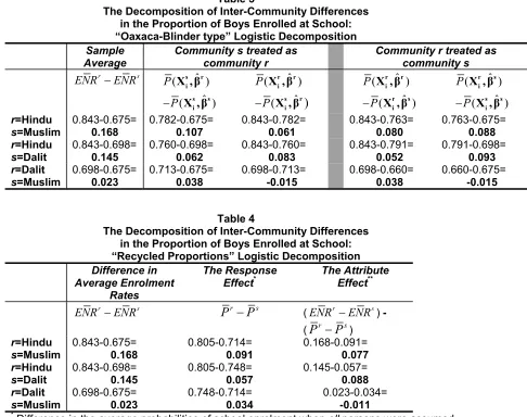
Table 3 shows the results from the ‘Oaxaca-Blinder’ logistic decompositions.

These show that, of the Hindu-Muslim difference in the mean enrolment rate

of boys, 64% - when Muslims were treated as Hindus (equation (3)) - and

48% - when Hindus were treated as Muslims (equation (4)) - could be

attributed to coefficient differences: these percentages reflected the

contribution of the ‘response effect’ towards explaining inter-community

differences in mean enrolment rates.

The response effect played a much smaller role in explaining differences in

mean enrolment rates between Hindus and Dalits: respectively, 43% of the

difference in the Hindu-Dalit enrolment rate for boys could be explained by

inter-community coefficient differences, when Dalits were treated as Hindus

(equation (3)); when Hindus were treated as Dalits (equation (4)), the

Although differences between Dalits and Muslims, in the mean enrolment

rates, were not as marked as between each of these communities and the

Hindus, this lack of difference concealed considerable differences between

Dalits and Muslims in terms of enrolment-enhancing attributes and attitudes.

Broadly speaking, Muslims were better endowed with enrolment-enhancing

attributes and qualitative evidence from the survey showed that Dalits had a

more positive attitude towards school participation. And this is seen clearly

when Muslim attributes were evaluated using Dalit coefficients: the mean

enrolment of Muslim boys rose from 68% to 71% (Table 3, right panel); on the

other hand, when Dalit attributes were evaluated using Muslim coefficients,

the mean enrolment of Dalit boys fell from 70% to 66% (Table 3, left panel).

Table 3 also makes clear that the proportion of the difference in mean

enrolment rates of boys, between Hindus and Muslims that could be ascribed

to inter-community coefficient differences, varied markedly (64%-48%)

depending upon whether Muslims were treated as Hindus (equation (3)) or

Hindus were treated as Muslims (equation (4)). A comparison of Hindu and

Dalit enrolment rates showed a similar variation (43%-36%).

The decomposition method suggested in this paper, as discussed earlier,

overcomes this difficulty. Table 4 shows that 54% of the difference between

the Hindu and Muslim average enrolment rates, and 39% of the difference

between Hindu and Dalit enrolment rates, for boys could be ascribed to the

“response effect”.

To what extent does the “attribute effect” contribute to the “response effect”?

Table 5 (using equation (12)) shows that 65% of the overall response effect,

between Hindus and Muslims, in the enrolment rate of boys was contributed

by the Central region and 27% was contributed by the Eastern region with the

percentage contributions of the ‘high enrolment rate regions’ of the South, the

West and the North being negligible. A similar story could be told with respect

to Dalits. This suggests that inter-community ‘attitudinal’ differences towards

the education of boys were, by and large, associated with the poorer regions

4. Conclusion

This paper has suggested a method of decomposing differences in

inter-group probabilities from a logit model and has shown how it might be viewed

as an extension of decompositions derived from the Oaxaca-Blinder

framework. In so doing, it has offered a solution to a problem, embedded

within the Oaxaca-Blinder decomposition, relating to the appropriate choice of

a common coefficient vector with which to evaluate the different attribute

vectors. This decomposition method also shows how pairwise comparisons

of groups might be conducted in the presence of more than two groups,

without discarding information on groups excluded from the comparison. This

is a particularly important consideration when applying decomposition

methods to investigating inter-group differences in economic circumstances in

pluralistic societies.

The decomposition technique was applied to examine inter-community

differences in India in the enrolment of boys at school. This gave rise to two

broad conclusions: first, that Muslims in India were better endowed with

enrolment-enhancing attributes but that Dalits had a more positive attitude

towards school enrolment. Second, that inter-community ‘attitudinal’

differences towards the education of boys were predominantly associated with

the poorer regions of India where the overall rate of school enrolment is very

low. These decomposition methods, therefore, also have important

implications for the causes of difference among ethnically diverse populations

References

Blackaby, D.H., Drinkwater, S., Leslie, D.G., Murphy, P.D. (1997), “A Picture of Male Unemployment Among Britain’s Ethnic Minorities”, Scottish Journal of Political Economy, vol. 44, pp. 182-197.

Blackaby, D.H., Leslie, D.G., Murphy, P.D. and O’Leary, N.C. (1998), “The Ethnic wage Gap and Employment Differentials in the 1990s: Evidence for Britain”, Economics Letters, vol. 58, pp. 97-103.

Blackaby, D.H., Leslie, D.G., Murphy, P.D. and O’Leary, N.C. (1999), “Unemployment Among Britain’s Ethnic Minorities”, The Manchester School, vol. 67, pp. 1-20.

Blinder, A.S. (1973), “Wage Discrimination: Reduced Form and Structural Estimates”, Journal of Human Resources, vol. 8, pp. 436-455.

Gomulka, J. and Stern, N. (1990), “The Employment of Married Women in the United Kingdom, 1970-83”, Economica, vol. 57, pp. 171-199.

Nielsen, H.S. (1998), “Discrimination and Detailed Decomposition in a Logit Model”, Economics Letters, vol. 61, pp. 115-20.

Oaxaca, R. (1973), “Male-Female Wage Differentials in Urban Labor Markets”, International Economic Review, vol. 14, pp. 693-709.

Data Appendix

The data used for estimating equation (13) were obtained from the NCAER

survey, referred to earlier. The salient features of this data are set out in this

section. The data from the NCAER survey are organised as a number of

‘reference’ files, with each file focusing on specific subgroups of individuals.

However, the fact that in every file an individual was identified by a household

number and, then, by an identity number within the household, meant that the

‘reference’ files could be joined – as described below – to form larger files.

So, for example, the schooling equations were estimated on data from the

‘individual’ file. This file, as the name suggests, gave information on the

194,473 individuals in the sample with particular reference to their educational

attainments3. From this file, data on the school enrolment of each male child

aged 6-14 were extracted (the variable ENR) and associated with this

information was data on: the educational attainments and occupation of the

boy’s father and/or mother; the income and size of the household to which the

boy belonged; the state, district and village in which he lived; his caste/tribe

(Dalit, non-Dalit); his religion; the number of his siblings etc. The equation

relating to school enrolment was estimated on data from the NCAER Survey's

‘Individual’ file’, described above, for boys between the ages of 6-14

(inclusive) who had both parents living in the household: this yielded a total of

19,845 observations.

Another file – the ‘village file’ – contained data relating to the existence of

infrastructure in, and around, each of the 1,765 villages over which the survey

was conducted. This file gave information as to whether inter alia a village:

had anganwadis4, primary schools, middle schools and high schools and, if it

did not, what was the nature of access to such institutions. The village file

could be joined to the individual file so that for each individual (say, boy

3

Needless to say, the file also contained other information on the individuals.

4

between 6-14) there was information not just on the his schooling outcome

and on his family and household circumstances but also on the quality of the

educational facilities – and general infrastructure - in the village in which he

lived.

The sample of children was distinguished by three mutually exclusive

subgroups: Dalits; Muslims; and Hindus. In effect, the Hindu/Muslim/Dalit

distinction made in this paper is a distinction between: non-Dalit Hindus;

Muslims; and Dalit Hindus . These subgroups are, hereafter, referred to as

‘communities’. Because of the small number of Christians and persons of

‘other’ religions in the Survey, the analysis reported in this paper was confined

to Hindus, Muslims and Dalits.

The Survey contained information for each of sixteen states. In this study, the

states were aggregated to form five regions: the Central region consisting of

Bihar, Madhya Pradesh, Rajasthan and Uttar Pradesh; the South consisting of

Andhra Pradesh, Karnataka, Kerala and Tamilnadu; the West consisting of

Maharashtra and Gujarat; the East consisting of Assam, Bengal and Orissa;

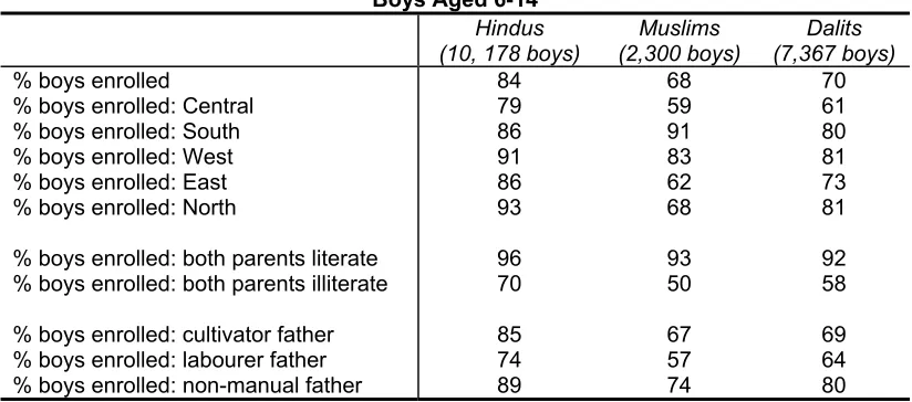
Table 1

Selected Data for School Enrolments by Community: Boys Aged 6-14

Hindus (10, 178 boys)

Muslims (2,300 boys)

Dalits (7,367 boys)

% boys enrolled 84 68 70

% boys enrolled: Central 79 59 61

% boys enrolled: South 86 91 80

% boys enrolled: West 91 83 81

% boys enrolled: East 86 62 73

% boys enrolled: North 93 68 81

% boys enrolled: both parents literate 96 93 92

% boys enrolled: both parents illiterate 70 50 58

% boys enrolled: cultivator father 85 67 69

% boys enrolled: labourer father 74 57 64

% boys enrolled: non-manual father 89 74 80

Table 2

Logit Estimates of the School Enrolment Equation: 19,845 Boys, 6-14 years

Determining Variables Coefficient Estimate (z value) Marginal Probabilities Muslim -0.4075898 (5.16) -0.160 Dalit -0.7991797 (2.49) -0.033 Central -0.5079733 (9.91) -0.100

South -

-West -

-East -0.6417705

(4.08)

-0.072

Household Income 1.002299

(3.01)

0.0003

Father educated: low 2.792598

(20.84)

0.128

Mother educated: low* 2.634748

(11.44)

0.113

Father educated: medium** 2.921865

(14.48)

0.121

Mother educated: medium** _2.114656

(5.14)

0.087

Father educated: high** 3.890858

(16.71)

0.148

Mother educated: high*** _2.1909003

(4.01)

0.089

Father cultivator 1.474474

(6.37)

0.056

Father labourer

-Father non-manual 1.550021

(7.45)

0.060

Mother Cultivator

-Mother labourer -0.7691638

(3.06)

-0.041

Mother non-manual -0.5848008

(3.22)

-0.092

No anganwadi in village -0.8018316 -0.032

(5.07)

No primary school in village

-No middle school within 2 km -0.8358139 (4.21)

-0.027

Number of Siblings -0.8985882

(7.20)

-0.016

Additional Effects of Muslims

Central -0.4962503

(4.10)

East -0.3896603

(4.80)

Father educated: medium 1.734144

(2.70)

Mother labourer 1.795181

(2.62)

Mother non-manual 6.466559

(2.41)

Anganwadi 1.739127

(4.40)

Middle School 1.508577

(3.55)

Number of Siblings 1.091813

(2.56)

Additional Effects of Dalits

Central -0.8562861

(1.71)

East -0.7160941

(2.38)

Father cultivator -0.8704603

(1.77)

Mother labourer 1.221465

(1.88)

Table 3

The Decomposition of Inter-Community Differences in the Proportion of Boys Enrolled at School: “Oaxaca-Blinder type” Logistic Decomposition

Sample Average

Community s treated as community r

Community r treated as community s

r s

ENR −ENR ( ˆ )

ˆ ( ) P P − s r i s s i

X ,β X ,β

ˆ ( ) ˆ ( ) P P − r r i s r i

X ,β X ,β

ˆ ( ) ˆ ( ) P P − r r i r s i

X ,β X ,β

ˆ ( ) ˆ ( ) P P − r s i s s i

X ,β X ,β

r=Hindu s=Muslim 0.843-0.675= 0.168 0.782-0.675= 0.107 0.843-0.782= 0.061 0.843-0.763= 0.080 0.763-0.675= 0.088 r=Hindu s=Dalit 0.843-0.698= 0.145 0.760-0.698= 0.062 0.843-0.760= 0.083 0.843-0.791= 0.052 0.791-0.698= 0.093 r=Dalit s=Muslim 0.698-0.675= 0.023 0.713-0.675= 0.038 0.698-0.713= -0.015 0.698-0.660= 0.038 0.660-0.675= -0.015 Table 4

The Decomposition of Inter-Community Differences in the Proportion of Boys Enrolled at School: “Recycled Proportions” Logistic Decomposition

Difference in Average Enrolment Rates The Response Effect* The Attribute Effect** r s

ENR −ENR Pr −Ps (ENRr −ENRs)

-(Pr −Ps)

r=Hindu s=Muslim 0.843-0.675= 0.168 0.805-0.714= 0.091 0.168-0.091= 0.077 r=Hindu s=Dalit 0.843-0.698= 0.145 0.805-0.748= 0.057 0.145-0.057= 0.088 r=Dalit s=Muslim 0.698-0.675= 0.023 0.748-0.714= 0.034 0.023-0.034= -0.011 *

Difference in the average probabilities of school enrolment when all persons were assumed to belong to community r against all persons belonging to community s

**

Calculated as the weighted sum of the individual Blinder-Oaxaca attribute effects (equation (8)).

Table 5

The Regional Contributions to the all-India “Response Effect”: Boys

Central South West East North All-India

Hindus v Muslims:

( H M)

m Pm Pm

µ − 0.059 0.003 0.002 0.024 0.003 0.091

Percentage contribution

65 3 2 27 3 100

Hindus v Dalits ( H M)

m Pm Pm

µ − 0.036 0.004 0.002 0.012 0.003 0.057

Percentage contribution

63 7 4 21 5 100