5
Performance Testing of RNSC and MCL Algorithms on
Random Geometric Graphs
Mousumi Dhara
Department of computer Engineering IIT (BHU),Varanasi
K. K. Shukla
Department of computer Engineering IIT (BHU), Varanasi
ABSTRACT
The exploration of quality clusters in complex networks is an important issue in many disciplines, which still remains a challenging task. Many graph clustering algorithms came into the field in the recent past but they were not giving satisfactory performance on the basis of robustness, optimality, etc. So, it is most difficult task to decide which one is giving more beneficial clustering results compared to others in case of real–world problems. In this paper, performance of RNSC (Restricted Neighbourhood Search Clustering) and MCL (Markov Clustering) algorithms are evaluated on a random geometric graph (RGG). RNSC uses stochastic local search method for clustering of a graph. RNSC algorithm tries to achieve optimal cost clustering by assigning some cost functions to the set of clusterings of a graph. Another standard clustering algorithm MCL is based on stochastic flow simulation model. RGG has conventionally been associated with areas such as statistical physics and hypothesis testing but have achieved new relevance with the advent of wireless ad-hoc and sensor networks. In this study, the performance testing of these methods is conducted on the basis of cost of clustering, cluster size, modularity index of clustering results and normalized mutual information (NMI) using both real and synthetic RGG.
General Terms
General Terms: Graph clustering, Data mining et. al.
Keywords
RNSC, MCL, Cost of clustering, Cluster size, NMI, RGG.
1.
INTRODUCTION
It is always expected that a complex system will be designed as a network. For example, a social network identifies relationships among mass of people like scientific community [1], movie actor collaborations [2], whereas biological networks denote interactions of molecules or proteins, the WWW [3] is moulded of web pages and hyperlinks, transportation [4] etc. Random graphs are often taking part to model these complex networks. The random geometric network is now-a-day getting immense popularity in society and nature for the complex system’s modelling.
Random geometric network models [5, 6] consist of a collection of entities called nodes embedded in a region of exclusively two or three dimensions, together with connecting links between pairs of nodes that exist with a probability related to the node locations. These models perform well in demonstrating numerous complex systems including Nano science [7], epidemiology [8, 9], forest fires [10], social networks [11, 12], and wireless communications [13–15].
To achieve some meaningful information about the network models and to visualize the details of the networks with many applications in a number of disciplines, clustering is necessary and it is more fruitful job than other ones. Graph clustering algorithms emphasis on clustering the nodes of a graph [16], [17]. It can expect from a graph clustering scenario that it contains a collection of sub graphs (nearly completely connected) and a small fraction of edges are existed between them for interconnection.
Recently, spectral clustering is getting immense popularity because of the convention of eigenvectors applied in various machine learning tasks [18]. In the recent past, various other graph clustering algorithms came into the field like restricted neighbourhood search clustering (RNSC) [19], Markov clustering (MCL) [20], super paramagnetic clustering (SPC), Genetic Algorithm, Molecular Complex Detection (MCODE), Local Clique Merging Algorithm (LCMA), etc.
RNSC, which is a cost based clustering method and executes local search iteratively to acquire optimum clustering in an efficient way. RNSC is a stochastic technique which uses restricted neighbourhood search concept. It also acts like a metaheuristic technique like tabu search, described in [21] and also can be used in various search space schematics. It is also known as Variable neighbourhood search [22]. The main goal of this algorithm is to discover the best cost clusterings (lower cost) from the set of clusterings of a graph by assigning some cost functions (Naive cost function and scaled cost function). The memory requirement for RNSC is O (n^2). The complexity of a move in the naive cost function is O (n), which is the size of the restricted neighbourhood of a move M.
MCL iscompetent clustering method for weighted graphs, based on the prototype of stochastic flow simulation technique. In this technique, clusters (a natural grouping of densely flow-connected vertices) are achieved by using two operators: flow expansion and inflation. MCL technique performs well for sparse graphs.
In this work, the performance of RNSC and MCL is verified on both real and synthetic benchmark random geometric graphs. Widespread experimental results on several real and synthetic datasets convey the detailedbehaviour of both the algorithms. The characteristics of both the algorithm are measured in terms of cost of clustering, cluster size, modularity index of clustering results and NMI value.
2.
GRAPH CLUSTERING ALGORITHMS
AND RANDOM GEOMETRIC GRAPH
6 RGG graph datasets, used in the performance analysis of these
algorithms.
2.1 RNSC (Restricted Neighbourhood
search clustering)
A.D. King introduced RNSC [19]as a local search meta-heuristic technique which is used to minimize the cost of clustering in the solution space. According to Stijn van Dongen, the vertex-wise performance criteria for clustering of unweighted graphs as the sum of the coverage measure taken on each vertex. Here, a simple integer-valued cost function (called the naive cost function) is taken as a pre-processor to generate initial clustering results on a graph and after that to estimate the low-cost clustering results, a more sensitive (but less effective) real-valued cost function (called the scaled cost function) is applied. The scaled function attempts to optimize the output from naive function and reach to the global optimal solution.
For a clustering C on a graph G (V, E) in which |V| = n, the coverage measure for Naïve cost function is stated as
1
( , , )
0( , , )
( , , ) 1
1
out
G C v
inG C v
Cov G C v
n
(1)Where
1out( , , )
G C v
and0
( , , )
in
G C v
are indicated respectively as a number of cross edges incident to v and number of vertices in Cv that are not adjacent to v and for agood clustering, these mentioned parameters should be small. Naive cost function is in the following expression.
1 0
1
( , )
(
( , , )
( , , ))
2
n out in
v V
C G C
G C v
G C v
(2)
The more sensitive scaled coverage measure is in the following expressionwhere, N (v) is the open neighbourhood of v.
1 0
( , , )
( , , )
( , , )
1
( )
out in
v
G C v
G C v
Cov G C v
N v C
(3) Now, the scaled cost function, built on scaled coverage measure is expressed as ineq (4), shown below.
1 0
1
1
( , )
(
( , , )
( , , ))
3
| ( )
|
s out in
v V v
n
C G C
G C v
G C v
N v
C
(4)2.2 MCL (Markov clustering)
To provide a very fast clustering technique, Stijn van Dongen, proposesMarkov Clustering algorithm which produces a natural group of clusterings for weighted graph [23]. This algorithm is established on the prototype of stochastic flow simulation technique using random walk. Two operators, flow expansion and inflation are used to generate a natural grouping of densely flow-connected vertices, which are called clusters. These two operators are constructed from the input graph and they are used to change the probability of the random walk as the Markov chain like way to another. Mainly, the inflation is used for strengthening the flow where it is strong and also weakening the flow where it is already weak and the flow expansion is used for propagating the flow
within the graph. MCL Algorithm is explained step by step below.
Step1: Input weighted directed or undirected graph; Step2: Create the adjacency matrix from the graph; Step3: Add self-loop to each vertex;
Step4: Normalize the matrix
R
k l ;Step5: Expand the matrix with eth power i.e.
(
R
kl)
eStep6: Inflate the matrix by taking inflation of the resulting matrix with parameter r;
Step7: Repeat step 5 and 6 until a steady state is achieved; Step8: Interpret resulting matrix to discover clusters.
The inflation operator is denoted as with power coefficient r, a real nonnegative number. The matrix is denoted as M
, M0.The matrix resulting from rescaling each of the columns of M with power coefficient r is denoted as i.e.
(5)
2.3 Random Geometric graph (RGG)
A random geometric graph [24] is denoted as G (n, r) where n is the number of nodes. The graph is constructed by inserting n points uniformly in terms of distribution at random on the unit square (or on the unit disk) and connecting two points if their Euclidean distance is at most the radius r (n). Generally, the set of vertices, represented as a set of random points which are generated by assigning n points uniformly at random in the unit square.In this random geometric graph the connection between two points is determined by using the distance parameter r which is the radius of the unitsquare orunit disk.
Now-a-days, this class of random graphs has gained importance as a natural model for wireless ad-hoc and sensor networks. Exploring properties of these random graphs can extract properties of the real-life systems they model and permit for the design of efficient algorithms. A pictorial representation of RGG is shownin fig1 with 500 nodes.
3. Few Parametric Concepts
r
k lR
rM
1 ( ) ( ) ( ) r pqr pq k
[image:2.595.308.533.566.737.2]r iq i M M M
7
3.1 Modularity Index
A topology-based modularity measure, basically proposed by Newman and Girvan [25], is used in this exploration to test the performance. This is a square symmetric matrix of clusters where each element dijdenotes the fraction of edges that link
nodes between clusters i and j and each diisignifies the
fraction of edges linking nodes within cluster i. The modularity measure is given by eq. (6).
2
( ii ( ij) )
i j
M
d
d (6)3.2 Normalized Mutual Information (NMI)
NMI measures the quality of clusters, which is the mutual information, shared between clusterings. This is mainly proposed by Alexander Strehl and JoydeepGhosh [26]. Let, there are set of groupings of clusterings as
which is indicated by ^. Let be the number of objects in cluster according to and be the number of objects in cluster according to . Let denotes the number of objects that are in according to and in cluster according to .The symbol is indicated as the assessment of NMI.
( ) ( )
( ) ( )
, , ( ) ( ) 1 1
( ) ( ) ( )
( ) ( )
( ) ( )
1 1
. log( )
( )
( log( ))( log( ))
a b
b a
k k h l
h l a b
h l
NMI a b h l
b a
k b k a
l h
l h
l h
n n n
n n
n n
n n
n n
(7)
3.3 Cluster Size
Cluster size can define the quality of clusters produced in clustering by any algorithm. It is also evaluate as the number of clusters, generated from the clustering results.
3.4 Graph size
It is obtained by computing the total number of nodes of the input graph. It is a basic parameter used in testing the behaviour of algorithms with different approach.
4. Experimental Results and Discussions
The efficiency and robustness of the RNSC and MCL algorithm are to be tested on few benchmark power-law graphs. To carry out the experiments, it needs real and synthetic data set as input of the algorithm. The performance of the algorithms will be verified by comparing the clustering results.All the experiments are carried out with the following initial configuration for RNSC and MCL. For RNSC, d (diversification Length) =10; D (shuffling Frequency) =40; t (tabu-length) =250 and e (number of experiments) =1000 and for MCL, the inflation value is 4; reweight loops c=0. 25; pre-inflation value p=0. 8 and preset resource scheme=5.
4.1 Evaluation on Synthetic RGG Graphs
Synthetic benchmark RGG graphs with increasing graph size are used for the performance evaluation of these graph clustering algorithms.
4.1.1 Cost of Clustering vsIncreasing Graph Size
for RNSC and MCL
This table contains the evaluated cost of clustering results, produced by RNSC and MCL. All the testing processes are conducted on RGG with increasing graph size.
Table1.Cost of Clustering with increasing Graph Size of RGG
Networks Cost of
Clustering (RNSC)
Cost of Clustering (MCL)
Geo500 32379.87 82929.31 Geo700 68444.88 162994.2
Geo900 107079.1 269100
Geo1100 158786.8 402413 Geo1500 295870.6 748134
Geo2000 533175.1 1332000
Fig 2: Cost of Clustering with Increasing Graph Size
Discussion: It is observed from figure 2 that the cost of
clustering of MCL is much higher than RNSC’s clustering results. The cost is measured for both the algorithms varying with increasing graph size of random geometric graph (RGG). The cost is increasing exponentially for both the case. But RNSC is giving less cost compared to MCL for RGG.
4.1.2
Modularity
of
Clustering
Resultsvs
Increasing Graph Size for RNSC and MCL
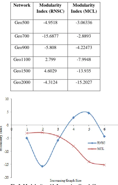
Table 2 gives the information about the entire computed modularity index of clustering results, produced by RNSC and MCL. All the testings are done on RGG with increasing graph size.
( )
{ q| {1,.., }}
q r
( )a h
n
h
c
( )a ( )b l nl
c
( )b,
h l
n
h
c
( )al
c
( )b
Table2. Modularity of Clustering with increasing Graph Size of RGG
Network Modularity
Index (RNSC)
Modularity Index (MCL)
Geo500 -4.9518 -3.06336
Geo700 -15.6877 -2.8893 Geo900 -5.808 -4.22473
Geo1100 2.799 -7.9948
Geo1500 4.6029 -13.935
[image:4.595.323.537.92.428.2]Geo2000 -4.3124 -15.2027
Fig 3: Modularity with Increasing Graph Size
Discussion: Modularity Index is an important measurement
technique to check the performance or accuracy of the clustering results of different graph clustering methods. It is shown in fig 3 that the modularity of RNSC’s clustering results is reaching to positive but it also decrease for some test cases. Modularity of MCL’s clustering shows that modularity is always decreasing to negative for all the test cases of RGG. So, RNSC is giving better clusterings compared to MCL.
4.1.3 Cluster Size vsIncreasing Graph Size for
RNSC and MCL
It is observed from table 3 that the evaluated cluster size from clustering process of RNSC and MCL are shown. These testing processes are conducted on RGG with increasing graph size.
Table3. Cluster size with increasing Graph Size of RGG
Network Cluster Size
(RNSC)
Cluster Size (MCL)
Geo500 166 375
Geo700 228 563
Geo900 293 714
Geo1100 350 843
Geo1500 478 1100
Geo2000 644 1565
Fig 4: Cluster Size with Increasing Graph Size
Discussion:It is observed from figure 4 that the cluster size of
MCL is increasing exponentially compare to RNSC’s cluster size for all the test cases. RNSC’s cluster size evaluation is getting significant position compared to MCL. RNSC is producing more accurate clusters compared to MCL. So, RNSC is giving more optimal and meaningful clusters compare to MCL.
[image:4.595.58.290.99.462.2]4.1.4 NMI ValuevsNumber of Experiments for
RNSC and MCL
[image:4.595.315.552.550.687.2]9
Discussion:The NMI value plays an important role in
checking the optimal nature of clusterings of different methods. It evaluates the algorithm’s behaviour in information passing through different clustering results. Fig 5 shows that the NMI value is high in case of RNSC compare to MCL. So the quality of the clusters of RNSC is better compared to MCL. After 300,500,700 runs with using real RGG graph (bork2455 [27]), the NMI value is obtained in case of RNSC and in case of MCL; experiments are performed by varying inflation value as I= {2.5, 3.5, 4.5}. The mutual information sharing between clusterings is more effective for RNSC whereas MCL can’t provide good quality clusters due to the less NMI value compare to RNSC. For all the three experiments, the NMI value of RNSC’s clustering is stable and in a much high position compared to the MCL’s NMI value of clustering results on real RGG.MCL is not giving accuracy in producing optimal clusters compared to RNSC.It can be concluded that RNSC is producing meaningful clusters compared to MCL’s produced clusters. So, RNSC is more optimal than MCL.
4.2 Evaluation on Real RGG Graphs
For this evaluation ‘bork2455’, 2002, high confidence yeast protein interactions by von Mering et al, is taken and the performance of these algorithms is tested on that graph. It is shown in the following table 1. The evaluated results shows that the cost of clustering produced by RNSC is lower compared to MCL. The computed modularity of clustering results of both the algorithm is produced and RNSC is gaining positive index whereas MCL is at negative index. RNSC’s cluster size evaluation is better compared to MCL. It is observed from the results, shown in table 1 that RNSC produces optimal clusters with lowering cost compared to MCL.
Table1. Clustering results of these algorithms on real RGG
Ne
two
rk
Co
st o
f
Clu
ste
rin
g
(
RN
S
C)
Co
st o
f
Clu
ste
rin
g
(
MCL)
Mo
d
u
la
rity
(
RN
S
C)
Mo
d
u
la
rity
(
MCL) Clu
ste
r
S
ize
(RN
S
C)
Clu
ste
r
S
ize
(M
CL)
bork24 55
121607.
5318
324408.
6402
13.
4137 -32.
4219
393 337
4.3 Visualization of Clustering of Real RGG
Bork and Synthetic Graphs
It is observed from figure7 and figure 8 that the clusters, evaluated by RNSC are more accurate and clearly visible compared to MCL’s evaluation. RNSC always produces meaningful clusters compared to MCL. Fig 7 and fig8 show the evaluated clustering of RNSC and MCL respectively on
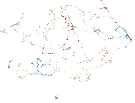
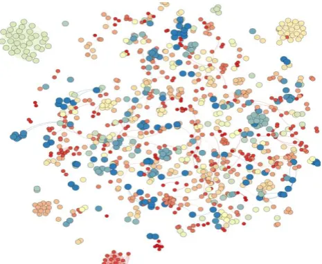
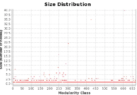
[image:5.595.308.542.273.740.2]bork2455 graph. For the real test graph, RNSC is performing better in producing clusters compared to MCL. It is obvious that RNSC is more optimal compared to MCL. Fig 6 shows the visual representation of real RGG bork2455.It is observed from this figure 6 that it is a complex network model with high protein interaction rate. Fig 9 shows the complex RGG network model with 1500 nodes. The nodes are randomly coordinated to form this complex network. Fig 10 and fig 11 show the size distribution graphs of clustering results, produced by RNSC and MCL respectively. The modularity is basically used to shrink the clustering result of these methods by similarity measures i.e. depend on various properties of a complex network. The figures show that RNSC is responding better in shrinking clustering results compared to MCL’s response to modularity. It can be concluded that the shrinking is done for RNSC better compared to MCL.
[image:5.595.316.549.537.728.2]Fig 7: Visualization of RNSC’s clustering Results on bork2455
Fig 8: Visualization of MCL’s clustering Results on bork2455
Fig 9: Synthetic RGG with1500 Nodes
5. CONCLUSIONS
This paper presents a comparative study between RNSC and MCL algorithm on RGG. Robustness and optimality of evaluated clustering results of RNSC and MCL algorithms are computed in terms of cost of clustering, modularity index of clustering results, cluster size and quality of clusters on the basis of NMI value. RNSC is getting better NMI value compared to MCL using real RGG. The quality of the clusters found in RNSC is better compared to MCL whereas MCL can find more number of clusters compared to RNSC. From the results, it is obvious that RNSC is more accurate than MCL. The cost curve shows that RNSC is producing lower-cost clustering results compared to MCL. The cluster size curve of MCL is increasing exponentially with increasing of graph size whereas RNSC is producing meaningful clusters for all the test graphs. It can be concluded that for both the case of real and synthetic benchmark RGG, RNSC is performing better compared to MCL in producing quality clusters with lowering cost. From the visualization, one’s attention can be attracted certainly on RNSC’s clustering results compared to MCL’s clustering on the real RGG graph. The time complexity of RNSC is O (n^3).The time complexity of MCL is O (n.k^2) where n is the number of nodes and k is the number of resources allocated per node. RNSC can be further extended by implementing it for weighted and directed graph where the weight can be added to the cost functions (naive and scaled cost), which will change and will give better results. Also, it can be further extended by a parallel move method which will give better results in the case of run-time or average cost. MCL can be further extended to produce good quality clusters.
6.
ACKNOWLEDGMENTS
The first author would like to thankfully acknowledge the research scholarship awarded by Banaras Hindu University, Varanasi.
[image:6.595.69.287.84.278.2]Fig 11: Modularity controlled clusters marking in MCL’s clustering on bork2455
[image:6.595.43.286.544.711.2]11
7.
REFERENCES
[1] Newman, M. E. J. 2001. Clustering and preferential attachment in growing networks. PhysicalReview E, 64:025102.
[2] Watts,Duncan J. and Strogatz,Steven H. 1998. Collective dynamics of ‘small-world’ networks. Nature, 393:440– 442.
[3] Huberman,Bernardo A. 1999. Growth dynamics of the World-Wide Web. Nature, 401:131.
[4] Amaral,L. A. N., Scala,A., Barth´el´emy,M., and Stanley,H. E. 2000. Classes of small-world networks. Proc. Natl. Acad. Sci. USA, 97:11149–11152.
[5] Penrose,M. 2003.Random Geometric Graphs (Oxford University Press, New York).
[6] Franceschetti,M. and Meester,R. 2007.Random Networks for Communication (Cambridge University Press, Cambridge, England).
[7] Kyrylyuk,V., Hermant,M. C., Schilling,T., Klumperman,B., Koning,C. E., and Schoot,P. van der 2011.Controlling electrical percolation in multicomponent carbon nanotube dispersions, Nature Nanotech. 6, 364-369.
[8] Miller,J. C., Soc.Roy, J.2009. Spread of infectious disease through clustered populations, Interf. 6, 1121 -1134.
[9] Danon,L., Ford,A. P., House,T., Jewell,C. P., Keeling,M. J., Roberts,G. O., Ross,J. V., and Vernon,M. C. 2011.Networks and the Epidemiology of Infectious Disease, Interdisc. Persp. Infect. Diseases, 284-909. [10]Pueyo,S., Grac¸a, P. M. L. D. A., Barbosa,R. I., Cots,R.,
Cardona,E., and Fearnside,P. M. 2010.Impact of boundaries on fully connected random geometric networks, Ecol. Lett. 13, 793.
[11]Palla,G., Barab´asi,A.-L, and Vicsek,T.2007.Quantifying social group evolution, Nature (London) 446, 664-667.
[12]Parshani,R., Buldyrev,S., andHavlin, S. 2011.Critical effect of dependency groups on the function of networks, Proc. Natl. Acad. Sci. 108, 1007.
[13]Haenggi,M., Andrews,J. G., Baccelli,F., Dousse,O., and Franceschetti,M.2009. Stochastic geometry and random graphs for the analysis and design of wireless networks, IEEE J. Select. Area. Commun. 27, 1029-1046.
[14]Li,J., Andrew,L. L. H., Foh,Zukerman,C. H., M., and Chen,H.-H. 2009. Connectivity, Coverage and Placement in Wireless Sensor Networks,Sensors, vol. 9, no. 10, pp. 7664-7693.
[15]Wang,P., Gonzalez,MC,Hidalgo, CA, Barabasi,A.-L2009. Understanding the spreading patterns of mobile phone viruses, Science 324, 1071-1076.
[16]Donath,W.E. and Hoffman,A.J.1973. Lower Bounds for the Partitioning of Graphs, IBM J. Research and Development, vol. 17, pp. 422- 425.
[17]Hall, K.M. 1970. An R-Dimensional Quadratic Placement Algorithm, Management Science, vol. 11, no. 3, pp. 219-229.
[18]Ng,A.Y., Jordan,M., and Weiss,Y.2001. On Spectral Clustering: Analysis and an Algorithm, Proc. 14th Advances in Neural Information Processing Systems (NIPS ’01).
[19]King,Andrew Douglas2004. Graph Clustering with Restricted Neighbourhood Search, M.S Thesis, University of Toronto.
[20]Dongen,S. M. van 2002. Graph Clustering by Flow Simulation. PhD thesis, University of Utrecht.
[21]Glover,F. 1989.Tabu search, part I. ORSA Journal on Computing, 1(3):190-206, summer.
[22]Mladenovi´c,N. and Hansen,P.1997. Variable neighbourhood search, Computers and Operations Research, 24(11):1097–1100.
[23]Dongen, S. M. van 2000. A cluster algorithm for graphs,Technical Report INS-R0010, Centrum voorWiskunde en Informatica.
[24]Penrose, M.D.2003. Random Geometric Graphs, Oxford Studies in Probability, OxfordU.P.
[25]Newman, MEJ and Girvan, M. 2004. Finding and evaluating community structure in networks, Physical Review E, 69, 026113–026127.
[26]Strehl, A. and Ghosh,J.2002. Cluster ensembles - a knowledge reuse framework for combining partitionings, AAAI, 93–98.