http://dx.doi.org/10.4236/jilsa.2014.64014
A Reinforcement Learning System to
Dynamic Movement and Multi-Layer
Environments
Uthai Phommasak1, Daisuke Kitakoshi2, Hiroyuki Shioya1, Junji Maeda1
1Division of Information and Electronic Engineering, Muroran Institute of Technology, Muroran, Japan 2Department of Information Engineering, Tokyo National College of Technology, Tokyo, Japan
Email: [email protected], [email protected], [email protected], [email protected]
Received 22 August 2014; revised 26 September 2014; accepted 8 October 2014
Academic Editor: Dr. Steve S. H. Ling, University of Technology Sydney, Australia
Copyright © 2014 by authors and Scientific Research Publishing Inc.
This work is licensed under the Creative Commons Attribution International License (CC BY). http://creativecommons.org/licenses/by/4.0/
Abstract
There are many proposed policy-improving systems of Reinforcement Learning (RL) agents which are effective in quickly adapting to environmental change by using many statistical methods, such as mixture model of Bayesian Networks, Mixture Probability and Clustering Distribution, etc. However such methods give rise to the increase of the computational complexity. For another method, the adaptation performance to more complex environments such as multi-layer envi-ronments is required. In this study, we used profit-sharing method for the agent to learn its policy, and added a mixture probability into the RL system to recognize changes in the environment and appropriately improve the agent’s policy to adjust to the changing environment. We also intro-duced a clustering that enables a smaller, suitable selection in order to reduce the computational complexity and simultaneously maintain the system’s performance. The results of experiments presented that the agent successfully learned the policy and efficiently adjusted to the changing in multi-layer environment. Finally, the computational complexity and the decline in effectiveness of the policy improvement were controlled by using our proposed system.
Keywords
Reinforcement Learning, Profit-Sharing Method, Mixture Probability, Clustering
1. Introduction
need to develop robotics software for learning and adapting to any environment. Reinforcement Learning (RL) is often used in developing robotic software. RL is an area of machine learning within the computer science do-main, and many RL methods have recently been proposed and applied to a variety of problems [1]-[4], where agents learn the policies to maximize the total number of rewards decided according to specific rules. In the process whereby agents obtain rewards; data consisting of state-action pairs are generated. The agents’ policies are effectively improved by a supervised learning mechanism using the sequential expression of the stored data series and rewards.
Normally, RL agents need to initialize the policies when they are placed in a new environment and the learn-ing process starts afresh each time. Effective adjustment to an unknown environment becomes possible by uslearn-ing statistical methods, such as a Bayesian network model [5] [6], mixture probability and clustering distribution [7] [8], etc., which consist of observational data on multiple environments that the agents have learned in the past [9] [10]. However, the use of a mixture model of Bayesian networks increases the system’s calculation time. Also, when there are limited processing resources, it becomes necessary to control the computational complexity. On the other hand, by using mixture probability and clustering distribution, even though the computational complexity was controlled and the system’s performance was simultaneously maintained, the experiments were only conducted on fixed obstacle 2D-environments. Therefore, examination of the computational complexity load and the adaptation performance in dynamic 3D-environments is required.
In this paper, we describe modifications of profit-sharing method with new parameters that make it possible to work on dynamic movement of multi-layer environments. We then describe a mixture probability consisting of the integration of observational data on environments that agent learned in the past within framework of RL, which provides initial knowledge to the agent and enables efficient adjustment to a changing environment. We also describe a novel clustering that makes it possible to select fewer elements for a significant reduction in the computational complexity while retaining system’s performance.
The paper is organized as follows. Section 2 briefly explains the profit-sharing method, the mixture probabil-ity, the clustering distribution, and the flow system. The experimental setup and procedure as well as the pres-entation of results are described in Section 3. Finally, Section 4 summarizes the key points and mentions our fu-ture work.
2. Preparation
2.1. Profit-SharingProfit-sharing is an RL method that is used as a policy learning mechanism in our proposed system. RL agents learn their own policies through “rewards” received from an environment.
2.1.1. 2D-Environments
The policy is given by the following function: :
w S× →A R (1) where S and A denote a set of state and action, respectively. Pair
( )(
s a, ∀ ∈ ∀ ∈s S, a A)
is referred to as a rule. w s a( )
, is used as the weight of the rule (w s a( )
, is positive in this paper). When state 0s is observed, a rule is selected in proportion to the weight of rule w s a
(
0, 0)
. The agent selects a single rule corresponding to given state 0s using the following probability:
(
0 0)
(
0(
0)
)
,
, ,
,
s S a A
w s a P s a
w s a
′∈ ′∈
=
′ ′
∑
(2) The agent stores the sequence of all rules that were selected until the agent reaches the target as an episode.(
)
(
)
{
1, 1 , , L, L}
L= s a s a (3)
where L is the length of the episode. When the agent selects rule
(
s aL, L)
and requires reward r, the weightof each rule in the episode is reinforced by
(
i, i)
(
i, i)
( )
( )
L if i =rγ − (5) where f i
( )
is referred to as the reinforcement function and γ ∈(
(
0,1]
)
is the “learning rate”. In this paper, the following nonfixed reward is used:(
)
0
r= + −r t n (6) where r0 is the initial reward, t is the action number limit in one trial and n is the real action number until
the agent reaches the target. We expect that the agent can choose a more suitable rule to reach the target in a dynamic environment by using this nonfixed reward.
2.1.2. 3D-Environments
The weight w s a
( )
, becomes w z s a(
, ,)
where z=1,,n (n is number of layers in this paper). The proba-bility of the rule(
z s a0, 0, 0)
becomes to this following function:(
0 0 0)
(
0(
0 0)
)
0 ,
, , , ,
, ,
s S a A w z s a P z s a
w z s a
′∈ ′∈
=
′ ′
∑
(7) and the new episode is given in the following function:(
) (
)
(
)
(
) (
)
(
)
(
) (
)
(
)
1 1
2 2
1 1 1 1 2 2 1
2 1 1 2 2 2 2
1 1 2 2
, , , , , , , , , , , , , , , , , , n n L L L L
n n n L L
z s a z s a z s a
z s a z s a z s a
z s a z s a z s a
=
(8)
1
n i i
L=
∑
= L (9) By the movement on z, we can set the pseudo-reward [11] by using the following function:(
) (
)
1, , , 0 1
n i
i z z
r =rγ − i= n <γ ≤ (10)
and update the weights according to the following function by using function (10):
(
i, j, j)
(
i, j, j)
( )
,w z s a ←w z s a + f i j (11)
( )
, Li j n i Li j(
1, ,)
, ( 1, , )i z i
f i j =rγ − =rγ γ− − i= n j= L (12)
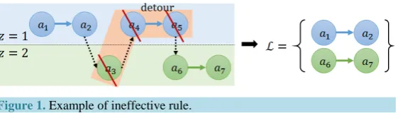
2.1.3. Ineffective Rule Suppression
As Figure 1, agent selects rule
(
z s1, L1,aL1)
in z1 then moves to z2. When agent selects any rule in z2 andfinally moves back to state
(
z s1, L1)
, the rules were selected on z2 are became detour rules which may notcontribute to the acquisition of the reward and these detour rules are called as ineffective rule[12] [13].
The ineffective rule has more negative effect such as the rules continue being selected repeatedly on the movement of z and agent cannot avoid from that situation. And this may make the policy learning become stagnation. From these reasons, the suppression of ineffective rule becomes necessary.
In this paper, we use this following method to suppress the ineffective rule:
Here, we use Li as the length of episode i and LC as a fixed number for determination ineffective rule.
When Li ≤LC∩zi−1=zi+1, all rules in i are decided to be ineffective rule. Here, all rules in i and the fi-
nal rule in i−1
(
zi−1,sLi−1,aLi−1)
will be excluded from as shown on Figure 1. 2.2. Mixture ProbabilityMixture probability is a mechanism for recognizing changes in the environment and consequently improving the agent’s policy to adjust to those changes.
Figure 1. Example of ineffective rule.
probabilistic knowledge about the environment. Furthermore, the policy acquired by the agent is improved by using the mixture probability of P ii
(
=1,,m)
obtained in multiple known environments. The mixing distri-bution is given by the following function:(
)
(
)
mix 1 , , , , m i i iP z s a βP z s a
=
=
∑
(13)where m denotes the number of joint distributions, and βi is the mixing parameter
(
∑
iβi =1,βi≥0)
. Byadjusting the environment subject to this mixing parameter, we expect appropriate improvement of the policy on the unknown dynamic environment.
In this paper, we use the following Hellinger distance [15] function to fix the mixing parameter:
(
)
( )
( )
1 2 2 1 1 2 2 ,H i i
x
D P Q = P x −Q x
∑
(14)where DH is the distance between Pi and Q, and DH is set to 0 when Pi and Q are the same. Pi is
joint distributions obtained in m different environments that an agent has learned in the past, Q is the sample distribution obtained from the successful trial of τ times in an unknown environment, and x is the total number of rules. Given that DH
(
P Qi,)
≤ 2 is established, the mixing parameter can be fixed by the following function:(
)
(
)
1 2 , 2 , H i i m H j jD P Q
D P Q
β = − = −
∑
(15)However, when
∑
mj=1 2−DH(
P Qj,)
=0, 1i m
β = , and when all distributions are equal, the mixing
para-meter is evenly allotted.
2.3. Clustering Distributions
We expect that the computational complexity of the system can be controlled and it will be possible to maintain the effectiveness of policy learning by selecting only the suitable joint distributions as the mixture probability elements based on this clustering method.
In this study, we used the group average method as opposed to the clustering method. The distance between the clusters can be determined by the following function:
(
)
(
)
, 1
, ,
i i j j
i j H i j
P Cl P Cl i j
D Cl Cl D P P
n n ∈ ∈
=
∑
(16)where n ni; j are the number of joint distributions contained in Cli and Clj, respectively. In this study, we
used the Hellinger distance function DH
(
P Pi, j)
. After completing the clustering, element Pi having themin-imum DH
(
P Qi,)
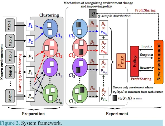
will be selected as the mixture probability element from each cluster. 2.4. Flow SystemFigure 2. System framework.
Step 1 Learn the policy in m environments by using the profit-sharing method to make the joint distribu-tions Pi = =
(
i 1,,m)
;Step 2 Cluster𝑚𝑚 distributions into n clusters;
Step 3 Calculate the Hellinger distance DH of distributions Pi and sample distribution Q;
Step 4 Select the element having the minimum DH
(
P Qi,)
from each cluster; Step 5 Calculate the mixing parameter βi;Step 6 Mix probability Pmix;
Step 7 Update the weight of all rules by using the following function:
new old old
mix
w ←w +w ×P (17) and then continue learning the updated weight by using the profit-sharing method.
3. Experiments
We performed an experiment to demonstrate the agent navigation problem and to illustrate the applied im-provement in the RL agent’s policy through the modification of parameters of the profit-sharing method and us-ing the mixture probability scheme. The purpose of this experiment was to evaluate the adjustment performance in the unknown dynamic 3D-environment by applying the policy improvement, and to evaluate its effectiveness by using mixture probability.
3.1. Experimental Setup
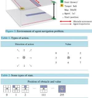
The aim in the agent navigation problem is to arrive at the target from the default position of the environment where the agent is placed. In the experiment, the reward is obtained when the agent reaches the target by avoid-ing the obstacle in the environment, as shown in Figure 3.
The types of state and action are shown in Table 1 and Table 2, respectively. Table 1 shows the output ac-tions of an agent in 8 direcac-tions and Table 2 shows 256 types of the total input states coming from the combina-tion of existing obstacles in 8 direccombina-tions. The 8 direccombina-tions are the top left, top, top right, left, right, bottom left, bottom, and bottom right. The agent has 2048 (8 actions × 512 states) rules in total that result from a combina-tion of input states and output accombina-tions in a layer. The size of agent, target, and environment are 1 × 1, 5 × 5, and 50 × 50, respectively.
3.2. Experimental Procedure
Figure 3. Environment of agent navigation problem.
Table 1. Types of action.
Direction of action Value
↑
← →
↓
0 1 2
3 4
5 6 7
Table 2. Some types of state.
Position of obstacle and value
… …
0 1 2 111 255
reaches the target at least once out of 200 action attempts. The action is selected by randomization and that ac-tion continues until the state is changed.
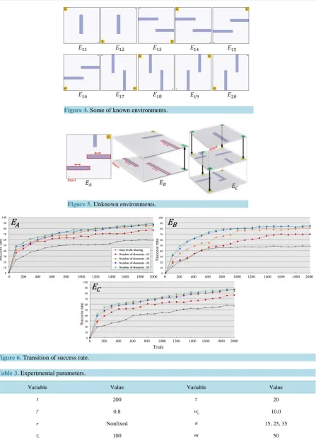
The purpose of the experiment is to learn the policy in unknown dynamic environments EA, EB and EC in
three cases (fixed obstacle, periodic dynamic and nonperiodic dynamic environments), by employing only the profit-sharing method and the mixture probability scheme (elements are m and n); the evaluation is based on the success rate of 2000 trials. The experimental parameters are shown in Table 3. Some of known environ-ments that became mixture probability eleenviron-ments, and the unknown dynamic environenviron-ments
(
E E EA, B, C)
usedto evaluate the policy improvement are shown in Figure 4and Figure 5, respectively. 3.3. Discussion
The success rate of policy improvement in EA, EB and EC by using only profit-sharing method and using
mixture probabilities and clustering is shown in Figure 6, and the processing time from Step 3 (system flow) until experiment finish in cases using all 50 elements and using only 35, 25 and 15 elements is shown in and Table 4, respectively
Figure 6 shows that the immediate success rate obtained by policy improvement is higher than that obtained by only the profit-sharing method in all environments. This means the speed of adaptation in unknown environ-ment is higher and the higher success rate continues until the experienviron-ments end. This results shows the success rate by policy improvement is higher than using only the profit-sharing more than 20% in EA and EC, and
more than 30% in EB. So, we can say the policy improvement is effective in all environments.
[image:6.595.154.452.119.436.2]Figure 4. Some of known environments.
[image:7.595.91.539.78.697.2]Figure 5. Unknown environments.
Figure 6. Transition of success rate.
Table 3. Experimental parameters.
Variable Value Variable Value
t 200 τ 20
γ 0.8 w0 10.0
r Nonfixed n 15, 25, 35
0
r 100 m 50
i
Table 4. Processing time.
Element number and processing time (s)
50 35 25 15
A
E 26.541 21.047 18.241 13.114
B
E 29.247 24.169 21.374 18.471
C
E 32.311 28.697 24.417 20.381
the success rate using all 50 elements was the highest, but that obtained using 25 elements was almost the same as that using all the elements in this result. So, the decline in effectiveness can still be controlled even if the number of mixture probability elements is reduced to half.
Furthermore, from the results in Table 4, we can see that by reducing the number of elements, the processing time was reduced considerably. Hence, we can say by using 25 elements, we can reduce the processing time without declining in policy improvement performance.
Figure 7 shows the typical trajectories of agent following the policy acquired while selecting data in envi-ronment EC in cases 1 - 500, 501 - 1000 and 1001 - 2000 trials. The intensity of color (from light red to dark
red) show the frequency of agent’s trajectories when they reached to target in each layers.
In these results, we can see in the first 500 trials, agent reached to all sub-targets in top layer. But due to the agent which started from sub-target 1 was the most difficult for reaching next sub-target, the number of time that agent reached to sub-target 1 became fewer in 501 - 1000 trials and finally almost reached to sub-target 2 and 3 in 1001 - 2000 trials. Also in middle layer, agent reached to all sub-targets in first 500 trials. But due to the agent which started from sub-target 5 was more easily for reaching to the final goal, the more number of trials there are, the more frequency of agent’s trajectories from sub-target 5 to the final goal increased clearly.
From the results of typical agent’, we can say by using the pseudo-reward, the agent can choose more suitable rules to reach the target in each layers even agent might be sometimes more difficult to reach in some layer, but more easily to reach to the final goal.
3.4. Supplemental Experiments
These experiments were conducted to compare the performance of the policy improvement in cases of fixed ob-stacle, periodic dynamic movement and nonperiodic dynamic movement on EA and EB by using 25 elements.
And experiments in only periodic and nonperiodic cases by using the same parameters were conducted 5 times.
4. Discussion
The results of policy improvement by using 25 elements of mixture probabilities in three cases are shown in Figure 8, and the results of five sets of experiments in periodic and nonperiodic dynamic movement are shown in Figure 9, respectively.
Figure 8 shows that the success rate in the case of periodic dynamic movement was almost no difference in the early period compared with the fixed obstacle case in both EA and EB, and continued to keep abreast of
high success rate until the experiments end. On the other hand, in the case of nonperiodic dynamic movement, even the success rate in EB was almost no difference or sometime was conversely higher compared with the
fixed obstacle case. However, as shown in Figure 9, even though the experiments were conducted by using the same parameters, the results of nonperiodic case in EA was quite low compared to periodic case. And the
re-sults of nonperiodic case were unstable in all EA and EB.
From these results, we can deduce that agent successfully learns the policy in the periodic dynamic movement environment and can more easily reach the target when the obstacle moves out from the trajectory as in EB. On
the contrary, when the obstacle moves into the trajectory, it will be more difficult for the agent to reach the tar-get.
5. Conclusions
Figure 7. Typical agent trajectories in EC.
[image:9.595.91.539.79.483.2]Figure 8. Transition of success rate (3 cases).
Figure 9. Five sets of experiments.
find the degree of similarity between the unknown and each known environment. We then used this as the basis to update the initial knowledge as being very useful for the agent to learn the policy in a changing environment. Even if obtaining the sample distribution is time-consuming, it is still worthwhile if the agent can efficiently learn the policy in an unknown dynamic environment.
Also, by using the clustering method to collect similar elements and then selecting just one suitable joint dis-tribution as the mixture probability elements from each cluster, we can avoid using similar elements to maintain a variety of elements when we reduce their number.
From the results of the computer experiment as an example application in the agent navigation problem, we can confirm that the policy improvement in dynamic movement environments is effective by using the mixture probabilities. Furthermore, agent is possible to select suitable rules to reach to the target in multi-layer by using the pseudo-reward. And the decline in effectiveness of the policy improvement can be controlled by using the clustering method. We conclude that the improvement of stability and speed in policy learning, and the control of computational complexity are effective by using our proposed system.
Acknowledgements
This research paper is made possible through the help and support by Honjo International Scholarship Founda-tion.
References
[1] Sutton, R.S. and Barto, A.G. (1998) Reinforcement Learning: An Introduction. MIR Press, Cambridge.
[2] Croonenborghs, T., Ramon, J., Blockeel, H. and Bruynooghe, M. (2006) Model-Assisted Approaches for Relational Reinforcement Learning: Some Challenges for the SRL Community. Proceedings of the ICML-2006 Workshop on Open Problems in Statistical Relational Learning, Pittsburgh.
[3] Fernandez, F. and Veloso, M. (2006) Probabilistic Policy Reuse in a Reinforcement Learning Agent. Proceedings of the Fifth International Joint Conference on Autonomous Agents and Multi-Agent Systems, New York, May 2006, 720- 727. http://dx.doi.org/10.1145/1160633.1160762
[4] Kober, J., Bagnell, J.A. and Peters, J. (2013) Reinforcement Learning in Robotics: A Survey. International Journal of Robotics Research, 32, 1238-1274. http://dx.doi.org/10.1177/0278364913495721
[5] Kitakoshi, D., Shioya, H. and Nakano, R. (2004) Adaptation of the Online Policy-Improving System by Using a Mix-ture Model of Bayesian Networks to Dynamic Environments. Electronics, Information and Communication Engineers,
104, 15-20.
[6] Kitakoshi, D., Shioya, H. and Nakano, R. (2010) Empirical Analysis of an On-Line Adaptive System Using a Mixture of Bayesian Networks. Information Science, 180, 2856-2874. http://dx.doi.org/10.1016/j.ins.2010.04.001
[7] Phommasak, U., Kitakoshi, D. and Shioya, H. (2012) An Adaptation System in Unknown Environments Using a Mix-ture Probability Model and Clustering Distributions. Journal of Advanced Computational Intelligence and Intelligent Informatics, 16, 733-740.
[8] Phommasak, U., Kitakoshi, D., Mao, J. and Shioya, H. (2014) A Policy-Improving System for Adaptability to Dynam-ic Environments Using Mixture Probability and Clustering Distribution. Journal of Computer and Communications, 2, 210-219. http://dx.doi.org/10.4236/jcc.2014.24028
[9] Tanaka, F. and Yamamura, M. (1997) An Approach to Lifelong Reinforcement Learning through Multiple Environ-ments. Proceedings of the Sixth European Workshop on Learning Robots, Brighton, 1-2 August 1997, 93-99.
[10] Minato, T. and Asada, M. (1998) Environmental Change Adaptation for Mobile Robot Navigation. 1998 IEEE/RSJ In-ternational Conference on Intelligent Robots and Systems, 3,1859-1864.
[11] Ghavamzadeh, M. and Mahadevan, S. (2007) Hierarchical Average Reward Reinforcement Learning. The Journal of Machine Learning Research, 8, 2629-2669.
[12] Kato, S. and Matsuo, H. (2000) A Theory of Profit Sharing in Dynamic Environment. Proceedings of the 6th Pacific Rim International Conference on Artificial Intelligence, Melbourne, 28 August-1 September 2000, 115-124.
[13] Nakano, H., Takada, S., Arai, S. and Miyauchi, A. (2005) An Efficient Reinforcement Learning Method for Dynamic Environments Using Short Term Adjustment. International Symposium on Nonlinear Theory and Its Applications, Bruges, 18-21 October 2005, 250-253.
[14] Hellinger, E. (1909) Neue Begrüündung der Theorie quadratischer Formen von unendlichvielen Veräänderlichen.
Journal für die Reine und Angewandte Mathematik, 136, 210-271.