http://dx.doi.org/10.4236/jpee.2014.29002
Calculation Method of Passive Residual Heat
Removal Heat Exchanger and Numerical
Simulation
Qiming Men, Xuesheng Wang, Xiang Zhou, Xiangyu Meng
Key Laboratory of Pressure Systems and Safety, Ministry of Education, East China University of Science and Technology, Shanghai, China
Email: [email protected]
Received May 2014
Abstract
The tube inside and outside heat transfer mechanism of Passive Residual Heat Removal Heat Ex-changer (PRHR HX) was analyzed. The calculation method of this special heat exEx-changer under natural convection condition in In-containment Refueling Water Storage Tank (IRWST) was car-ried out. The single-tube coupling model three-dimensional natural circulation in the IRWST was simulated numerically using Fluent. The heat transfer and flow characteristics of the fluid in IRWST were obtained. The comparison of the results between theoretical arithmetic and numeri-cal simulation showed that the theoretinumeri-cal numeri-calculation method is suitable for the heat transfer numeri- cal-culation of PRHR HX.
Keywords
Passive Residual Heat Removal Heat Exchanger, Heat Transfer Calculation Method, Numerical Simulation, Natural Convection
1. Introduction
The passive residual heat removal heat exchanger (PRHR HX) removes core decay heat to mitigate loss of heat sink events depressurizes the system [1]. It transfers heat from the primary side to the containment by heating the water in the in-containment refueling water storage tank (IRWST). The PRHR HX consists of a C-shaped heat exchanger tube bundle submerged in the IRWST [2] [3].
calculation methods of PRHR HX at present.
Yonomoto [4] carried out an experimental investigation to simulate small-break loss-of-coolant accidents in the reactor using the ROSA-V Large-scale Test Facility. The three-dimensional natural circulation in the IRWST was simulated numerically using the Fluent code. The total heat transfer rate and the fluid temperature distribution in the IRWST of the PRHR HX were predicted well according to their investigation. Pan Xinxin [5] conducted a numerical investigation of AP600 PRHR HX with Fluent and obtained the temperature distribution of IRWST at different times. The transient numerical results show that the heat transfer performance is consis-tent with AP600 experimental data. A similar investigation was conducted by Xue Ruojun [6] which described a lot of visual mechanism. In the earlier investigation, only the flow and temperature distribution in IRWST was investigated, the flow in tube was not considered.
This paper describes the heat transfer calculation method of PRHR HX. Then a numerical simulation of sim-plified coupling model is conducted to verify the method.
2. Calculation Method
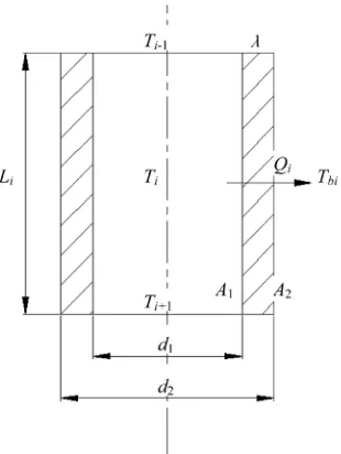
Inspired by the finite element idea, the heat exchanger tube is virtually divided into several calculation cells. It-erative calculation is carried out in each cells to get the wall heat flux, the heat transfer coefficients and tem-perature along the tube. Figure 1 shows the calculation model diagram of the i’th cell. The follow assumptions are considered in the calculation:
1) Fluid temperature is uniform in the radial direction, only changes in the axial direction of IRWST (which can be confirmed in the numerical simulation section);
2) Heat transfer performance of different tube is the same. The central tube (average tube length) of tube bun-dle is analyzed;
3) Fluid temperature distribution along the vertical direction of IRWST is a known factor; 4) All these parameters in the i’th cell is the average value of the cell inlet and outlet; 5) The fouling resistance is not considered.
The heat transfer in PRHR HX is an unsteady process, but at a certain moment the changes in temperatures and flow rate are negligible. So it can be considered as a quasi-steady state at the moment. The heat transfer rate from the i’th cell to the IRWST fluid can be obtained from the quasi-steady-state one dimensional equation of heat transmission.
1
( )
i p i i
Q =Wc T− −T (1)
where
[image:2.595.238.393.497.703.2]W = tube inside fluid mass flow rate, kg/s;
cp = tube inside fluid constant pressure heat capacity, J/(kg·K); Ti-1, Ti = tube inside fluid temperature of the i − 1’th and i’th cell, K;
The heat transfer in PRHR HX can be divided into three stages: convection heat transfer from tube inside fluid to tube inside wall, heat conduction from tube inside wall to outside wall and convection heat transfer from tube outside wall to fluid in IRWST [7]. Heat conduction in fluid is not considered. The heat flux of the i’th cell can be expressed as:
( )
(
)
1 1
i i i wi i
Q =A⋅πd l T − T (2)
( ) ( )
(
2 1)
2
ln
wi i wo i
i i
T T
Q l
d d
πλ −
= (3)
( )
(
)
2 2
i i wo i bi
Q = A ⋅πd l T −T (4)
According to Equations (2)-(4), the following expression can be obtained:
(
)
2
1 1 1 2 2
1 1 1
ln 2
i i bi i
l T T
Q
d
d A d d A
π λ − = + + (5) where
li = length of the i’th cell, m;
Tbi = tube outside fluid temperature of the i’th cell, K; λ = thermal conductivity of the tube material, W/(m∙K); d1 = inner diameter of the tube, m;
d2 = outer diameter of the tube, m;
A1 = heat transfer coefficient on the inner surface of the tube, W/(m2∙K); A2 = heat transfer coefficient on the outer surface of the tube, W/(m2∙K).
The first cell fluid temperature (T0) which equals to the tube inlet fluid temperature of the heat exchanger is a known value. Then the outlet fluid temperature (T1) of the first cell can be obtained through Equation (1) and Equation (5). T1 is then used as the inlet fluid temperature of the second cell to calculate T2. Then the tube inside fluid temperature distribution along the heat exchanger tube can be obtained. The heat flux, the tube inner wall temperature and tube outer wall temperature can also be obtained.
As mentioned above, the value of heat transfer coefficient on the inner and outer surface of the tube should be known to get the heat flux. So the proper empirical correlations calculating the heat transfer coefficients need to be determined. In consider of present investigation only simulates natural convection in IRWST and the heat exchanger tube is a vertical tube, the unrelated correlations are not mentioned in this paper.
Inner surface heat transfer correlation.
The Reynolds numbers of the internal flow were fully turbulent range (Re > 6000) according to the flow rates and fluid temperatures. The heat transfer on the inner surface is therefore calculated by using the Dittus-Boelter [7] correlation for the turbulent forced convection flow:
0.8 1/3 1 0.023 Re Pr
k A
d
= (6)
where
k = fluid thermal conductivity, W/(m∙K); d = inner diameter of tube, m;
Re = Reynolds number; Pr = Prandtl number.
This correlation is available in many handbooks such as [7]. The fluid physical properties are evaluated with the average temperature in each cells.
Outer surface heat transfer correlation
( LPr)n hl
Nu C Gr
k
= = (7)
where
Nu = Nusselt number; GrL = Grasof number,
3 2
L
Gr =gβ∆Tl ν ;
l = characteristic length, equals tube length for vertical tube, m; g = local gravitational acceleration, m/s2;
T
∆ = temperature difference between tube outside wall temperature and environment temperature, K; β = coefficient of volume expansion, 1/K;
ν = kinematic viscosity, Pa∙s.
Coefficient C and n are experimental parameters, the value and applicability of the two parameters can be found in [8]. The fluid physical properties are evaluated with the average temperature of wall temperature and environment temperature.
3. Numerical Simulation of the Single Tube Model
3.1. Geometry Model and Meshing
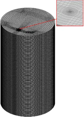
In order to simplify the computation and shorten the calculation time, the vertical tube model throughout the water tank was adopted to calculate, and the tank size was scaled down. The model was meshed with ICEM CFD and Gambit. The total elements of the grid are 48.8W, the whole and partial mesh is shown in Figure 2.
3.2. Model Assumptions and Solving Settings
In order to simplify calculation and save the calculation time without affecting the calculation results, the fol-lowing assumptions were considered:
1) The value of the tube inlet temperature is constant;
2) The upper, lower surface and the side wall of Water tank are adiabatic; 3) The impact of automatic sprinkler system in IRWST is not considered; 4) The Boussinesq assumption describing natural convection is used.
The single-tube coupling model was numerically studied with FLUENT 12.1. The k-ε turbulence model is ap-plied to simulate fluid flow in tube and tank. The standard wall function and the full effects of buoyancy were considered.
[image:4.595.243.385.503.700.2]As there are no subcooled boiling models in Fluent, it is impossible to simulate subcooled boiling to verify the formula of subcooled boiling heat transfer. The natural convection model in fluent is employed to verify the heat
transfer calculation method.
Tubes inlet is velocity-inlet boundary, and the temperature is set to 95˚C. The export is outflow boundary. The upper, lower surface and the side wall of Water tank are considered adiabatic. Coupling surface using shell conduction was given wall thickness 1.65 mm. The initial temperature of tank is set to 5˚C.
3.3. Temperature Field Analysis
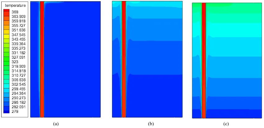
The temperature distribution of the tank center surface, at 120 s, 1010 s and 2560 s, is shown in Figure 3. As can be seen, at the initial heating stages (t = 120 s), the liquid temperature around the tubes increases firstly. Be-cause the heat of the tube inside fluid transmits to the water tank through the wall, the surrounding liquid starts to be heated and the temperature rises rapidly. After that, natural convection flow caused by the temperature difference appears in the tank. Then the fluid moves upward along the heat exchange tube under the effect of buoyancy lift and the upper cooling water get heated. The fluid temperature stratified phenomenon appears in the tank. The phenomenon proves that the assumption “water temperature in the radial direction (horizontal di-rection) the same, only in the axial direction (vertical didi-rection) change” is reasonable.
3.4. Flow Analysis
The tank flow chart of the cross sectional at 20 s, 1010 s and 2560 s were shown in Figure 4. From this figure, the flow distribution is very similar at the three moments. At the beginning of heating, fluid flow to the top of the tank along the outer surface of the heat exchange tube. On the upper surface of the tank, fluid flows to the opposite tank wall, then flow down along the tank wall. The vortex forms in this process, and the size and posi-tion of the vortex changes as time goes on. This made the fluid mixture well in the tank and is conducive for enhancement of the heat transfer capability.
4. Results and Discussion
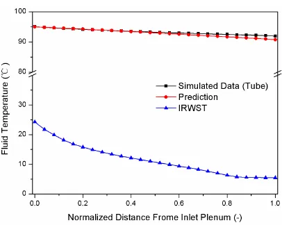
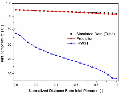
The numerical simulated fluid temperatures along the centre line of the IRWST at three different times (120 s, 1010 s and 2560 s) were exported to calculate the tube inside fluid temperatures using the calculation method mentioned above. The calculated tubes inside temperatures were then compared to the simulated data. The comparison result is shown in Figure 5-7. The Y-axis was broken to obtain a pleasant appearance of the figures.
In these figures, “Simulated Data” represents the numerical simulated tube inside fluid temperatures which are the average tube fluid temperature at different levels. “Prediction” represents the tube inside fluid tempera-tures calculated with the calculation method. “IRWST” represents the fluid temperature distribution along the centre line of IRWST.
[image:5.595.87.512.500.707.2]
(a) (b) (c)
[image:6.595.119.481.81.274.2]
(a) (b) (c)
[image:6.595.210.416.305.461.2]Figure 4. Path line of center surface in different moments. (a) t = 120 s; (b) t = 1010 s; (c) t = 2560 s.
Figure 5. Comparison of calculation results at 120 s.
Figure 6. Comparison of calculation results at 1010 s.
[image:6.595.212.415.484.646.2]Figure 7. Comparison of calculation results at 2560 s.
5. Conclusions
1) The heat transfer calculation method of PRHR HX is proposed. The heat exchanger tube is virtually di-vided into several calculation cells. Iterative calculation is carried out in each cell to get the wall heat flux, the heat transfer coefficients and temperature along the tube.
2) A numerical simulation of simplified coupling model is conducted. Fluid flow and temperature distribution in IRWST under natural convection condition is investigated. The assumptions proposed in the calculation method are confirmed according to the simulated results.
The numerical simulation data is used to test and verify the calculation method. The results show that the er-ror is acceptable, the calculation method is correct and can be used for the heat transfer design and checking calculation of PRHR HX.
References
[1] Tower, S.N., Schulz, T.L. and Vijuk, R.P. (1988) Passive and Simplified System Features for the Advanced Westing-house 600 MWe PWR. Nuclear Engineering and Design, 109, 147-154.
http://dx.doi.org/10.1016/0029-5493(88)90153-7
[2] Schuulz, T.L. (2006) Westinghouse AP1000 Advanced Passive Plant. Nuclear Engineering and Design, 236, 1547- 1557. http://dx.doi.org/10.1016/j.nucengdes.2006.03.049
[3] Reyes J.N., et al. (1998) Scaling Analysis for the OSU AP600 Test Facility (APEX). Nuclear Engineering and Design,
186, 53-109. http://dx.doi.org/10.1016/S0029-5493(98)00218-0
[4] Yonomoto, T., Kukita, Y. and Schuliz, R.R. (1998) Heat Transfer Analysis of the Passive Residual Heat Removal Sys-tem in ROSA/AP600 Experiments. Nuclear Tech, 124, 18-30.
[5] Pan, X.X. (2010) Numerical Study and Sensitivity Analysis of PRHR HX Transient Heat Transfer Performance.
Nu-clear Power Engineering, 31, 97-102.
[6] Xue, R.J., Deng, C.C. and Peng, M.J. (2010) Numerical Simulation Research of Natural Convection Heat Exchanger. Asia-Pacific Power and Energy Engineering Conference, Chengdu, 1-5.
[7] Pitts, D. and Sissom, L. (1997) Theory and Problems of Heat Transfer. 2nd Edition, McGraw-Hill, New York.