INVESTIGATIONS INTO THE COGNITIVE ABILITIES OF ALTERNATE LEARNING CLASSIFIER SYSTEM ARCHITECTURES

(1)

University of Kentucky University of Kentucky

UKnowledge

University of Kentucky Doctoral Dissertations Graduate School

2006

INVESTIGATIONS INTO THE COGNITIVE ABILITIES OF

ALTERNATE LEARNING CLASSIFIER SYSTEM ARCHITECTURES

David Alexander Gaines

University of Kentucky, [email protected]

Right click to open a feedback form in a new tab to let us know how this document benefits you. Right click to open a feedback form in a new tab to let us know how this document benefits you.

Recommended Citation Recommended Citation

Gaines, David Alexander, "INVESTIGATIONS INTO THE COGNITIVE ABILITIES OF ALTERNATE LEARNING CLASSIFIER SYSTEM ARCHITECTURES" (2006). University of Kentucky Doctoral Dissertations. 250. https://uknowledge.uky.edu/gradschool_diss/250

(2)

ABSTRACT OF DISSERTATION

The Graduate School

University of Kentucky

(3)

INVESTIGATIONS INTO THE COGNITIVE ABILITIES OF ALTERNATE LEARNING CLASSIFIER SYSTEM ARCHITECTURES

A dissertation submitted in partial fulfillment of the requirements for the degree of Doctor of Philosophy in the

College of Business and Economics at the University of Kentucky

By

Lexington, Kentucky

Director: Dr. Ramakrishnan Pakath, Professor of DSIS and Gatton Endowed Research Professor

Lexington, Kentucky

2006

(4)

The Learning Classifier System (LCS) and its descendant, XCS, are promising paradigms for machine learning design and implementation. Whereas LCS allows classifier payoff predictions to guide system performance, XCS focuses on payoff-prediction accuracy instead, allowing it to evolve “optimal” classifier sets in particular applications requiring rational thought. This research examines LCS and XCS performance in artificial situations with broad social/commercial parallels, created using the non-Markov Iterated Prisoner’s Dilemma (IPD) game-playing scenario, where the setting is sometimes asymmetric and where irrationality sometimes pays. This research systematically perturbs a “conventional” IPD-playing LCS-based agent until it results in a full-fledged XCS-based agent, contrasting the simulated behavior of each LCS variant in terms of a number of performance measures. The intent is to examine the XCS paradigm to understand how it better copes with a given situation (if it does) than the LCS perturbations studied.

Experiment results indicate that the majority of the architectural differences do have a significant effect on the agents’ performance with respect to the performance measures used in this research. The results of these competitions indicate that while each architectural difference

significantly affected its agent’s performance, no single architectural difference could be credited as causing XCS’s demonstrated superiority in evolving optimal populations. Instead, the data suggests that XCS’s ability to evolve optimal populations in the multiplexer and IPD problem domains result from the combined and synergistic effects of multiple architectural differences.

In addition, it is demonstrated that XCS is able to reliably evolve the Optimal Population [O] against the TFT opponent. This result supports Kovacs’ Optimality Hypothesis in the IPD

environment and is significant because it is the first demonstrated occurrence of this ability in an environment other than the multiplexer and Woods problem domains.

(5)

KEYWORDS: Genetic Algorithms, Classifier Systems, Machine Learning, Iterated Prisoner’s Dilemma, Cognitive Aspects

(6)

By

Ramakrishnan Pakath Director of Dissertation

Merl M. Hackbart Director of Graduate Studies

(7)

RULES FOR THE USE OF DISSERTATIONS

Unpublished dissertations submitted for the Doctor’s degree and deposited in the University of Kentucky Library are as a rule open for inspection, but are to be used only with due regard to the rights of the author. Bibliographical references may be noted, but quotations or summaries of parts may be published only with the permission of the author, and with the usual scholarly

acknowledgements.

Extensive copying or publication of the dissertation in whole or in part also requires the consent of the Dean of the Graduate School of the University of Kentucky.

A library that borrows this dissertation for use by its patrons is expected to secure the signature of each user.

(8)

DISSERTATION

The Graduate School University of Kentucky

(9)

DISSERTATION

A dissertation submitted in partial fulfillment of the requirements for the degree of Doctor of Philosophy in the

College of Business and Economics at the University of Kentucky

By

Lexington, Kentucky

Director: Dr. Ramakrishnan Pakath, Professor of DSIS and Gatton Endowed Research Professor

Lexington, Kentucky

2006

(10)

(11)

ACKNOWLEDGMENTS

This research benefited from the efforts of many, the most significant of which was the tireless and unceasing support and encouragement I received from my dissertation advisor, Dr.

Ramakrishnan Pakath. In the five years I’ve known Ram, he has served as a true example of all that is right regarding higher education, not only for me, but for countless undergraduate and graduate students. He is a credit to his profession and I am fortunate for having been able to work with him.

I am also very fortunate to have had an excellent and supportive dissertation committee made up of Dr. Clyde Holsapple, Dr. Cidambi Srinivasan, Dr. Chen Chung, and Dr. Timothy Smith. Drs. Srinivasan and Holsapple, in particular, were especially generous with their time, knowledge, and support as I wound my way through the research process.

I am also grateful to the UK gang: Kiku Jones, Dan Davenport, Partha Mohaptra, Lei Chi, Dave Kroger, Dennis Pearce, Sharath Sasidharan, Matt Seevers, Haeran Jae, Shannon Rinaldo; and to the DFM gang: Vern Francis, Jim Parco, Randy Blass, Steve Green, Rita Jordan, Kurt Heppard, Steve Fraser, Eric Holt, and Andy Armacost, for providing much needed support and motivation during the entire journey.

Finally, it goes without saying that I could not have finished my doctoral saga without the love, support, understanding, and occasional kick in the butt I received from my immediate family, Darcy, Conor, and Katie, as well as from my lifelong heroes Marty and Gary Gaines. The final obligatory nod goes to the ever-present alter ego, Leonard Leibowitz, for keeping it real.

(12)

TABLE OF CONTENTS

Acknowledgments...iii

List of Tables...viii

List of Figures...x

List of Equations...xi

Chapter I: Introduction...1

A. Overview ...1

B. Relevant Literature Review ...2

(1) Learning Classifier Systems ...2

(2) The Prisoner’s Dilemma ...3

(3) Prior Experimental Evidence...4

C. Methodology ...4

D. Results ...7

E. Contributions and Limitations ...8

(1) Contributions...8

(2) Limitations ...9

Chapter II: Review of the Literature...10

A. Introduction...10

B. Artificial Intelligence ...10

(1) Background and Definition...10

(2) Artificial Intelligence Families...11

(3) Artificial Intelligence Strategies...13

(a) Overarching Strategy...14

(b) Representation...14

(c) Supervision ...14

(4) Machine Learning ...15

(a) Learning by Rote...16

(b) Learning from Instruction ...16

(c) Learning by Analogy ...16

(d) Learning from Examples...17

(e) Learning from Observation and Discovery...18

C. Learning Classifier Systems...18

(1) LCS-0: A “Traditional” Learning Classifier System...19

(a) LCS-0 Architecture...19

i. Rule and Message Subsystem...21

ii. Apportionment of Credit Subsystem ...23

iii. Classifier Discovery Mechanisms...29

(b) Genetic Algorithm ...30

i. Selection...32

ii. Crossover...32

iii. Mutation...33

(c) Replacement and Crowding...34

(d) Classifier Systems: The Holistic Viewpoint...35

(e) Other Mechanisms ...39

(13)

(f) Applications of Classifier Systems and Genetic Algorithms ...40

(g) Shortcomings of the traditional LCS algorithm...41

(h) Summary...42

(2) XCS: An Extended Classifier System...42

(a) Overview...43

(b) XCS Architecture and Major Cycle ...43

i. Matching and the Match Set ...44

ii. The Prediction Array and Action Set ...44

iii. Executing the Action and Updating the Action Set...45

iv. Initial Population and Covering ...47

v. Genetic Algorithm...47

(c) Summary ...48

D. IPD: The Experimental Testbed ...48

(1) The Prisoner’s Dilemma ...49

(2) The Iterated Prisoner’s Dilemma ...52

(a) IPD Players...53

i. RAND...54

ii. CCC ...54

iii. DDD ...54

iv. TFT (Tit for Tat) ...54

v. TFTT (Tit for Two Tats) ...54

vi. TTFT (Two Tits for Tat) ...54

vii. GTFT (Generous Tit for Tat) ...55

viii. JOSS (Joss’s Strategy)...55

ix. FRDM (Friedman’s Strategy)...55

(b) Benefits ...55

(c) Limitations...57

(3) Experimental Testbed Rationale...57

Chapter III: Methodology...61

A. Simulation...61

(1) Agent-Based Simulation...62

(2) Rationale...62

B. Experiments ...62

(1) Goals...63

(a) Complete Payoff Map...63

i. Complete...64

ii. Accurate ...64

iii. Minimal ...64

iv. Non-overlapping ...64

(b) Maximally General Classifiers ...65

i. Over-general...66

ii. Maximally General...66

iii. Sub-optimally General ...66

(2) Prior Research ...66

(3) Differences Between LCS and XCS...68

(a) The Key Difference...68

(b) Population Differences...68

(14)

i. Initial Population ...68

ii. Population Size ...68

(c) Genetic Algorithm Differences ...69

i. GA Scope...69

ii. Parent Selection ...69

iii. Classifier Deletion ...69

(d) Action Selection...70

(e) Classifier Updates ...70

(4) Generating Perturbations...70

(5) Performance ...70

(a) Learning vs Steady State Phases ...71

(b) Measures ...72

i. Performance ...72

iii. Problem Difficulty...73

iv. System Error ...74

v. Learning Rate ...74

vi. Statistical Tools...74

vii. Other Possible Measures...75

(6) Experiment Suite and Propositions ...75

(a) The Key Difference...77

(b) Population Differences...77

i. Initial Population ...77

(c) Genetic Algorithm Differences ...78

i. GA Scope...78

ii. Parent Selection ...78

iii. Classifier Deletion ...78

(d) Action Selection...79

(e) Classifier Updates ...79

(7) Methodological Issues...79

C. Conclusion...80

Chapter IV: Experimental Findings and Analysis...81

A. Versus TFT ...82

(1) Number of Unique Classifiers ...82

(a) Order of Stabilization...85

(b) Magnitude at Stabilization...85

(c) Learning Rate ...86

(2) % Correct Responses ...87

(3) System Error...92

(4) % of Optimal Population [O] ...97

(15)

(a) Order of Stabilization... 100

(b) Magnitude at Stabilization... 100

(c) Learning Rate ... 101

B. Versus RAND... 102

(1) Number of Unique Classifiers ... 102

(2) % Correct Responses ... 107

(3) System Error... 112

(4) % of Optimal Population [O] ... 117

C. Proposition Testing... 117

(1) The Key Difference... 117

(2) Population Differences ... 118

(a) Initial Population ... 118

(b) Population Size... 119

(3) Genetic Algorithm Differences ... 121

(a) GA Scope... 121

(b) Parent Selection... 122

(c) Classifier Deletion ... 123

(4) Action Selection ... 124

(5) Classifier Updates... 124

D. Conclusions ... 125

Chapter V: Conclusions ... 127

A. Contributions... 127

B. Limitations... 128

C. Future Research... 129

D. Summary ... 130

Appendix A: Coding the Program in Visual Basic.NET ... 131

Appendix B: XCS Sets and Parameters ... 134

Appendix C: Program Code Listing... 136

Appendix D: SAS Statistical Tests Output ... 273

Appendix E: Charts, Graphs, and Plots ... 293

References... 323

Vita... 329

(16)

LIST OF TABLES

Table I-1 Key Architectural Differences...5

Table I-2 Agent vs Opponent Competitions...7

Table II-1 Samples of Valid Classifiers...22

Table II-2 Classifier Bid Variables...25

Table II-3 Classifier Strength Variables...27

Table II-4 Biological and Artificial Vernacular Correspondence ...30

Table II-5 Classifier System Extensions...40

Table II-6 Engineering Applications of Genetic Algorithms...40

Table II-7 Applications of Classifier Systems...40

Table II-8 Prisoner’s Dilemma Reward Structure...50

Table III-1 Sample Payoff Landscape ...65

Table III-2 Sample Classifiers ...66

Table III-3 TFT Optimal Population ...73

Table III-4 Competitions Between Agents and Opponents ...76

Table IV-1 Descriptive Characteristics, Unique Classifiers vs TFT...84

Table IV-2 Rank-Ordered Stabilization Encounter versus TFT WRT Unique ...85

Table IV-3 Rank-Ordered Stabilized Means versus TFT WRT Unique ...86

Table IV-4 Rank-Ordered Learning Rate versus TFT WRT Unique ...87

Table IV-5 Descriptive Characteristics, % Correct vs TFT ...89

Table IV-6 Rank-Ordered Stabilization Encounter versus TFT WRT % Correct...90

Table IV-7 Rank-Ordered Stabilized Means versus TFT WRT % Correct...91

Table IV-8 Rank-Ordered Learning Rate versus TFT WRT % Correct...92

Table IV-9 Descriptive Characteristics, System Error vs TFT...94

Table IV-10 Rank-Ordered Stabilization Encounter versus TFT WRT System Error...95

Table IV-11 Rank-Ordered Stabilized Means versus TFT WRT System Error...96

Table IV-12 Rank-Ordered Learning Rate versus TFT WRT System Error...96

Table IV-13 Descriptive Characteristics, % [O] vs TFT ...99

Table IV-14 Rank-Ordered Stabilization Encounter versus TFT WRT % [O] ... 100

Table IV-15 Rank-Ordered Stabilized Means versus TFT WRT % [O] ... 101

Table IV-16 Rank-Ordered Learning Rate versus TFT WRT % [O] ... 101

Table IV-17 Descriptive Characteristics, Unique Classifiers vs RAND... 104

Table IV-18 Rank-Ordered Stabilization Encounter versus RAND WRT Unique ... 105

Table IV-19 Rank-Ordered Stabilized Means versus RAND WRT Unique ... 106

Table IV-20 Rank-Ordered Learning Rate versus RAND WRT Unique ... 107

Table IV-21 Descriptive Characteristics, % Correct vs RAND ... 109

Table IV-22 Rank-Ordered Stabilization Encounter versus RAND WRT % Correct ... 110

Table IV-23 Rank-Ordered Stabilized Means versus RAND WRT % Correct ... 111

Table IV-24 Rank-Ordered Learning Rate versus RAND WRT % Correct ... 111

Table IV-25 Descriptive Characteristics, System Error vs RAND ... 114

Table IV-26 Rank-Ordered Stabilization Encounter versus RAND WRT System Error... 115

Table IV-27 Rank-Ordered Stabilized Means versus RAND WRT System Error... 116

Table IV-28 Rank-Ordered Learning Rate versus RAND WRT System Error... 116

Table IV-29 Accuracy-Based Fitness: Unique Classifiers vs TFT and RAND ... 117

Table IV-30 Accuracy-Based Fitness: % [O] vs TFT and RAND ... 118

Table IV-31 Initial Populations: Learning Rates vs TFT and RAND ... 118

(17)

Table IV-32 Initial Populations: Unique Classifiers vs TFT and RAND... 119

Table IV-33 Population Size: Learning Rates vs TFT and RAND... 120

Table IV-34 Population Size: Unique Classifiers vs TFT and RAND ... 120

Table IV-35 GA Scope: Learning Rates vs TFT and RAND ... 121

Table IV-36 GA Scope: % Correct vs TFT and RAND ... 121

Table IV-37 GA Scope: System Error vs TFT and RAND... 122

Table IV-38 Parent Selection: Unique Classifiers vs TFT and RAND ... 122

Table IV-39 Parent Selection: % Correct vs TFT and RAND... 122

Table IV-40 Parent Selection: System Error vs TFT and RAND... 123

Table IV-41 Parent Selection: Learning Rates vs TFT and RAND... 123

Table IV-42 Classifier Deletion: % [O] vs TFT and RAND ... 123

Table IV-43 Action Selection: % Correct vs TFT and RAND ... 124

Table IV-44 Action Selection: System Error vs TFT and RAND ... 124

Table IV-45 Action Selection: Learning Rates vs TFT and RAND ... 124

Table IV-46 Classifier Updates: Learning Rates vs TFT and RAND... 125

(18)

LIST OF FIGURES

Figure I-1 Simulation Experiment Program User Interface...6

Figure II-1 Artificial Intelligence Family Tree...12

Figure II-2 Classes of Techniques That Contain Learning Classifier Systems ...13

Figure II-3 General Reinforcement Learning Framework ...17

Figure II-4 Interactions between Classifier System and Environment...20

Figure II-5 Traditional Learning Classifier System Modules...21

Figure II-6 Auction in Classifier System ...26

Figure II-7 Simple Genetic Algorithm Flowchart...31

Figure II-8 Classifier System and Environment Interactions: Application Mode...35

Figure II-9 Classifier System and Environment Interactions: Learning Mode...35

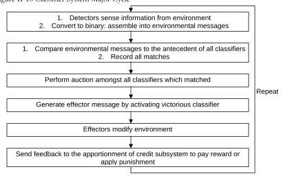
Figure II-10 Classifier System Major Cycle...36

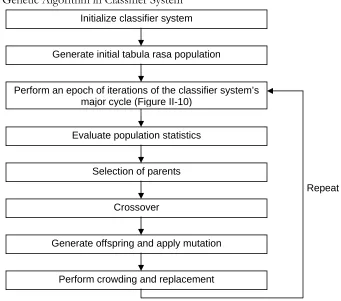
Figure II-11 Genetic Algorithm in Classifier System ...37

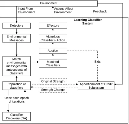
Figure II-12 The Classifier System and Interaction with Environment: Learning Mode ...38

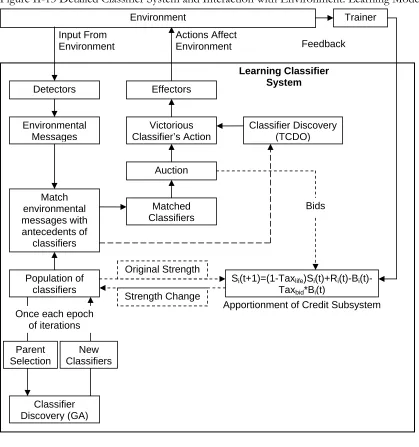
Figure II-13 Detailed Classifier System and Interaction with Environment: Learning Mode ...39

Figure II-14 XCS Architecture...44

Figure IV-1 Unique Classifiers vs TFT ...83

Figure IV-2 % Correct vs TFT ...88

Figure IV-3 System Error vs TFT...93

Figure IV-4 % [O] vs TFT ...98

Figure IV-5 Unique Classifiers vs RAND... 103

Figure IV-6 % Correct vs RAND ... 108

Figure IV-7 System Error vs RAND ... 113

(19)

LIST OF EQUATIONS

Equation II-I Calculation of Classifier’s Bid...24

Equation II-II Calculation of Classifier’s Effective Bid...26

Equation II-III Calculation of Classifier’s Strength...27

Equation II-IV Calculation of Inactive Classifier’s Strength After n Iterations...28

Equation II-V Calculation of Taxlife Rate ...28

Equation II-VI Calculation of Classifier’s Strength...29

Equation II-VII Calculation of Classifier’s Selection Probability...32

Equation II-VIII XCS Update Function...45

Equation II-IX XCS Recency Weighting ...46

Equation II-X XCS Error Update Function ...46

Equation II-XI XCS Accuracy Update Function ...46

Equation II-XII XCS Relative Accuracy Function...46

Equation II-XIII XCS Fitness Update Function ...47

Equation II-XIV Prisoner’s Dilemma Reward Property #1...49

Equation II-XV Prisoner’s Dilemma Reward Property #2...50

(20)

CHAPTER I: INTRODUCTION

A. OVERVIEW

Well before the HAL 9000 entered the collective consciousness in Stanley’s Kubrick’s 1968 movie, “2001: A Space Odyssey,” people were intrigued with Artificial Intelligence (AI) and its potential applications. Intelligent machines in movies, from 2001’s HAL 9000 to Terminator’s liquid metal cyborg to Star Wars’ R2D2 and C3 PO have accelerated the interest in AI, wowing and inspiring us to dream of a day when machines are our equals. The appeal is so strong that one of AI’s pioneers suggested that: “… AI can be defined as the attempt to get real machines to behave like the ones in the movies” (Allen 2001).

The idea of teaching a machine to behave as a human is alluring, both for practical and for more esoteric reasons. Imagine having a machine at your disposal to perform your day’s mundane tasks, and to do them as well as or better than you. Science has made significant strides in this regard, producing intelligent machines that use genetic algorithms to help manage airport logistics, that use intelligent text parsing to find and organize job openings, that use robotic machines to survey and sanitize the battlefield, and that use neural networks to recognize fraudulent credit card activity (Kahn 2002).

In many areas, however, progress has been disappointing, and in a way, surprising to many experts. Marvin Minsky, the head of the AI laboratory at MIT, proclaimed in 1967 that “within a generation the problem of creating Artificial Intelligence will be substantially solved” (Minsky 1967). About the same time, Herbert Simon, another prominent computer scientist, announced that by 1985 “machines will be capable of doing any work that a man can do” (Simon 1965). That’s hardly the attitude today. In fact, by 1982 Minsky was admitting, “The AI problem is one of the hardest science has ever undertaken” (Kolata 1982).

This research, then, furthers the state of AI knowledge in a direction many believe to be the most promising area for AI, Machine Learning. One expert states emphatically that “Machine Learning is the most important aspect of AI” and that the ability to continually learn and adapt is central to intelligence. (Waltz 2000). This research furthers knowledge in this area by examining a currently popular mechanism for adaptation in Machine Learning, the Learning Classifier System (LCS) and one of its variants, known as XCS. Through experimentation with these algorithms, this research contributes to the ongoing discourse about intelligent machines and their ability to learn. A

(21)

thorough review of the literature indicates that research with the focus and setting chosen here has not been attempted before. Therefore, the findings from this research are unique and value-adding to the existing body of knowledge on unsupervised learning systems.

B. RELEVANT LITERATURE REVIEW

(1) Learning Classifier Systems

The concept behind Learning Classifier Systems is simple; an excellent description is provided by Wilson (Wilson 1994):

A classifier system is a learning system in which a set of condition-action rules called classifiers competes to control the system and gain credit based on the system’s receipt of reinforcement from the environment. A classifier’s cumulative credit, termed strength, determines its influence in the control competition and in an evolutionary process using a genetic algorithm in which new, plausibly better, classifiers are generated from strong existing ones, and weak classifiers are discarded.

This description may be broken down into the primary determinants of an LCS: • Learning system

• Set of condition-action rules

• Competition and cooperation to control system

• Operation based on reinforcement from the environment • Evolutionary processes

• Plausibly better classifiers which are generated from strong existing ones • Removal of weak classifiers

The first classifier system of note was Cognitive System One (CS-1), developed by John Holland and Judith Reitman in 1978 (Holland and Reitman 1978). CS-1 ran a simulated linear maze with external payoff only at the maze ends, so that the correct step-direction had to be learned at each interior point. From these modest beginnings, LCS-based algorithms have been intensely researched and applied to a wide variety of environments (Wilson and Goldberg 1989).

The most recent incarnation of the LCS paradigm, known as XCS, was originally proposed by Stewart Wilson in 1995. XCS, or eXtended LCS, differs primarily in its calculation of classifier

(22)

fitness and in the scope of its genetic algorithm. In XCS, classifier fitness is based on the accuracy of a classifier’s payoff prediction instead of the magnitude of the payoff. In addition, the genetic

algorithm takes place in XCS’s Action Sets instead of in the population as a whole. XCS has been shown to work better than traditional Learning Classifier systems in certain environments (Wilson 1995). The current research dissects the differences between XCS and earlier variants of Learning Classifier Systems to discern the key determinants of XCS’s performance in a new experimental environment.

(2) The Prisoner’s Dilemma

The new environment under study in the current research is the Iterated Prisoner’s Dilemma (IPD) game-playing scenario. Because of its broad implications and applicability, the IPD has been widely studied and applied as a model for interactions between individuals and organizations. In the current research, the IPD is appealing because it is inherently non-Markov, sometimes asymmetric, and one where irrationality sometimes outperforms rationality. These characteristics are explained in greater detail in Chapter II: D. (2) and result in the IPD being particularly challenging to an artificial player. The IPD game also has broader commercial and social parallels than prior LCS settings explored. Although it has received sustained research scrutiny since the 1950s, research momentum exploded after Axelrod’s (Axelrod 1984) pioneering efforts in applying evolutionary systems to outwit humans. The impetus continues, as evidenced by recent announcements by the United Kingdom’s Engineering and Physical Sciences Research Council (EPSRC) (2003; 2005). The EPSRC announced it was co-hosting a series of competitions into the latest developments surrounding the Iterated Prisoner’s Dilemma and was specifically inviting researchers to best the winner in Axelrod’s original IPD competitions. In the present research, the IPD game serves as a useful and novel test-bed for studying Learning Classifier System behavior.

In the Prisoner’s Dilemma (PD), two players can either cooperate (C) or defect (D). If both cooperate or both defect, each receives a reward of R2 or R3, respectively. If one defects while the other cooperates, the latter gets a sucker’s payoff of R₄ while the former gets R₁. Here,

R1>R2>R3>R4 and (R1+R4)/2<R2. Thus, while mutual cooperation is preferred to mutual defection (R2>R3), individual defection is tempting (R1>R2; R3>R4), and repeated cooperation is more lucrative than each alternately playing sucker. Therein lies the dilemma: on any given move, should a player cooperate or defect? In an Iterated PD, players repeatedly play one another and therefore may be able to exploit prior experience with an opponent.

(23)

(3) Prior Experimental Evidence

Despite advances in LCS methods and techniques, direct comparison of traditional LCS

algorithms with the XCS algorithm is hard to find. Most research comparing the two approaches has been focused on their relative performance in learning the Boolean multiplexer functions and in finding goals in grid-like “woods” and maze environments (Wilson 1999). While useful and

illuminating, these results leave much room for speculation regarding XCS’s purported advantages. Although preliminary efforts have been made to quantify performance differences between LCS- and XCS-based algorithms (Kovacs 2000), comparison of XCS with strength-based classifier systems remains one of the top 5 priorities of future XCS research (Wilson 2003).

Moreover, traditional LCS-based systems have been shown to perform very well in some settings, such as evolving novel fighter aircraft maneuvering patterns (Smith, Dike et al. 2000; Smith, Dike et al. 2000). Thus, it would appear that the traditional LCS model is not entirely without merit, and should therefore not be discarded as a viable Machine Learning technique (Wilson 1999).

Extant research with Learning Classifier Systems and the IPD is limited. Noteworthy examples include Smith and Dike, et al.’s work with fighter aircraft maneuvering, in which the authors make the argument that a one-versus-one fighter aircraft scenario is analogous to the IPD (Smith, Dike et al. 2000), Chalk and Smith’s experimentation with various learning classifier system parameters in an IPD environment (Chalk and Smith 1997), and Meng and Pakath’s suite of simulation experiments using a traditional LCS in the IPD (Meng and Pakath 2001). These efforts do not investigate the performance of XCS in the IPD environment and specifically do not include a comparison of LCS and XCS in such a setting. This research, therefore, is novel in both its setting and in its approach. C. METHODOLOGY

This research compares and contrasts traditional LCS-based algorithms with an XCS algorithm under specific IPD tournament settings to (a) better understand their adaptive behaviors, and (b) determine to what extent the purported virtues of XCS hold in more complex settings like the IPD.

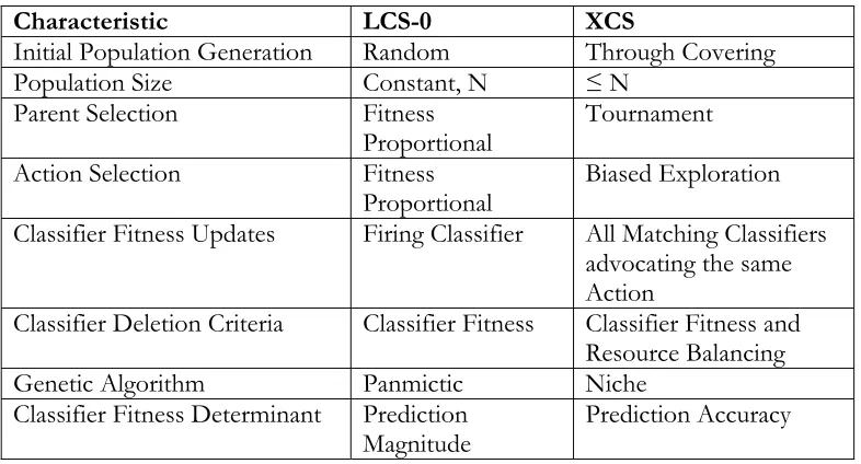
Using simulation experiments, the learning and steady-state behavior characteristics of a modern IPD-playing XCS-based adaptive agent (XCS) are repeatedly compared with those of a series of LCS-based agents beginning with a “traditional” model (LCS-0), followed by agents that differ from LCS-0 in only one key architectural characteristic. In each comparison, both agents play against the same IPD opponent(s). This approach draws on the following key architectural

differences between LCS-0 and XCS.

(24)

Table I-1 Key Architectural Differences

Characteristic LCS-0 XCS

Initial Population Generation Random Through Covering

Population Size Constant, N ≤ N

Parent Selection Fitness

Proportional

Tournament

Action Selection Fitness

Proportional Biased Exploration Classifier Fitness Updates Firing Classifier All Matching Classifiers

advocating the same Action

Classifier Deletion Criteria Classifier Fitness Classifier Fitness and Resource Balancing

Genetic Algorithm Panmictic Niche

Classifier Fitness Determinant Prediction

Magnitude Prediction Accuracy

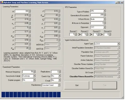
To investigate the effect of these architectural differences, a custom simulation experiment program was coded in Visual Basic.NET. The final source code listing has approximately 6,500 lines and provides for the selection of both the learning agent and its opponent, as well as for the setting of various experimental and simulation parameters. In addition, the program incorporates routines to collect relevant performance data for later analyses. The following screen capture provides a view of the simulation program’s user interface.

(25)

Figure I-1 Simulation Experiment Program User Interface

The initial competitions were conducted between LCS-0, the traditional LCS-based agent, and each of two pre-programmed IPD-playing opponents. The purpose of these competitions was to establish baseline performance characteristics against which to compare subsequent competitions.

Subsequent competitions were held between the two pre-programmed IPD-playing opponents and LCS-based agents which differed in one way from the traditional LCS agent. Because only one characteristic was changed in each of these competitions, performance differences were necessarily due to the effects of changing that unique characteristic.

The final competitions were held between a full blown XCS learning agent and the same two pre-programmed opponents used in previous competitions. Because XCS employs all of the architectural differences and is theorized to provide superior performance to LCS, these final competitions provided a theoretical upper bound to learning agent performance.

Ultimately, the following twenty competitions were held:

(26)

Table I-2 Agent vs Opponent Competitions Competition

Number

Agent and Architectural Characteristics Opponent

1 TFT 2

LCS-0 (Baseline LCS)

RAND

3 TFT 4

LCS-1 (Initial Population: Random

→Through Covering) RAND

5 TFT 6

LCS-2 (Population Size: Constant, N →≤

N) RAND

7 TFT 8

LCS-3 (Parent Selection: Fitness

Proportional → Tournament) RAND

9 TFT 10

LCS-4 (Action Selection: Fitness

Proportional → Biased Exploration) RAND

11 TFT 12

LCS-5 (Classifier Fitness Update: Firing

Classifier → All Classifiers in [A]) RAND

13 TFT 14

LCS-6 (Classifier Deletion Criteria: Fitness

Only → Fitness and Resource Balancing) RAND

15 TFT 16

LCS-7 (Genetic Algorithm: Panmictic →

Niche) RAND

17 TFT 18

LCS-8 (Classifier Fitness Determinant:

Magnitude → Accuracy) RAND

19 TFT 20

XCS

RAND

D. RESULTS

Statistical analyses of the data generated during these experiments indicate that the majority of the architectural differences did have a significant effect on the agents’ performance with respect to the performance measures used in this research. The results of these competitions indicate that while each architectural difference significantly affected its agent’s performance, no single architectural difference could be credited as causing XCS’s demonstrated superiority in evolving optimal populations. Instead, the data suggests that XCS’s ability to evolve optimal populations in the multiplexer and IPD problem domains result from the combined and synergistic effects of multiple architectural differences.

In addition, it was demonstrated that XCS was able to reliably evolve the Optimal Population [O] against the TFT opponent. This result supports Kovacs’ Optimality Hypothesis in the IPD environment and is significant because it is the first demonstrated occurrence of this ability in an environment other than the multiplexer and Woods problem domains.

(27)

It is therefore apparent that while XCS performs better than its LCS-based counterparts, its demonstrated superiority may not be attributed to a single architectural characteristic. Instead, XCS’s ability to evolve optimal classifier populations in the multiplexer problem domain and in the IPD problem domain studied in this research results from the combined and synergistic effects of multiple architectural differences.

E. CONTRIBUTIONS AND LIMITATIONS

(1) Contributions

As described previously, the current research is noteworthy because it has not been attempted previously and therefore offers new insight into the workings of LCS and XCS. Stewart Wilson, the designer and architect of XCS and a well-regarded authority in the field, commented that the current research was “… very important …” and “… will reveal some interesting architectural and

performance data about LCS and XCS, and perhaps more importantly, will take XCS into new territory that should have wide application” (Wilson 2005).

In addition, several specific features of this work distinguish it from prior research with Learning Classifier Systems:

1. This research constitutes the first known decomposition and study of the XCS algorithm’s constituent parts. Specifically, eight significant architectural differences between traditional LCS and XCS systems were identified and analyzed. While each architectural characteristic was shown to significantly affect performance, none in and of itself could be credited as providing XCS’s demonstrated superiority. Instead, it is apparent that XCS’s ability to evolve optimal populations in the multiplexer, woods, and IPD problem domains is due to the combined and synergistic effects of multiple architectural differences.

2. The Iterated Prisoner’s Dilemma is a new and previously untested problem domain for XCS-based systems. This domain is unique because it is not a static or deterministic domain as are the previously studied multiplexer and woods environments. Moreover, depending on the opponent, IPD competitions often call for irrational decision making, challenging learning agents in new and previously untested ways. The IPD also has broader social and business parallels than do previously studied environments, offering greater ability to extend and apply research results. Other benefits of the IPD problem domain include asymmetric updates of the knowledge base and the ability to test learning agents against multiple opponents, including “noisy,” changing, or illogical opponents.

(28)

3. This research provides the first demonstration of XCS’s ability to reliably evolve the

Optimal Population [O] against the TFT opponent. This result supports Kovacs’ Optimality Hypothesis in the IPD environment and is significant because it is the first demonstrated occurrence of this ability in an environment other than the multiplexer and Woods problem domains.

4. To accomplish this research, a computer simulation program was written in Visual Basic.NET, the first known instance of such a program in this language. VB.NET offers several advantages over other languages used in previous classifiers system research. First, it is executable on common Windows-based personal computers, greatly extending the flexibility of the researcher. Second, VB.NET modules may be written to integrate program execution with other Windows-based programs, providing the ability for automatic data capture and display. This feature is employed in the current research, with modules to automatically store and display data in Microsoft Excel spreadsheets. VB.NET also offers the ability to interact with the user in a visual manner, providing the researcher with the ability to examine evolutionary path traces during the course of normal execution. This ability is employed in the current research and greatly aided the researcher in tracking classifiers throughout the evolution process.

(2) Limitations

LCS- and XCS-based learning agents are complex mechanisms with many moving parts; the lack of understanding regarding these parts provides much of the impetus for the current research. As an example, the XCS implementation relies on over 20 parameters in its execution (an exposition of these parameters is provided in Appendix B: XCS Sets and Parameters). Historically, parameter values have been set relying as much on intuition as on empirical research. This research relies on these generally accepted values for these parameters, necessarily limiting its results to a specific set of parameter values. Second, as described later in this paper, there exist many possible competitions between learning agents and pre-programmed opponents. This research studies competitions between the learning agents and a select subset of these opponents, again limiting the generality of the results. Third, the LCS-based learning agents used in this research differ in only one way from the traditional LCS implementation. Combining architectural differences in a systematic manner would provide additional information regarding cumulative effects and offers the possibility of increased insight into the workings of LCS and XCS algorithms.

(29)

CHAPTER II: REVIEW OF THE LITERATURE

A. INTRODUCTION

Learning Classifier Systems and its more recent variants is one of many techniques belonging to the field of Artificial Intelligence. This chapter, therefore, provides an introduction to AI and

Machine Learning, particularly as these fields relate to the current research. This introduction to AI is followed by a description of a traditional Learning Classifier System and its more recent variant, the eXtended Classifier System. Finally, the chosen testbed for this research, the Iterated Prisoner’s Dilemma, is explained and detailed. The purpose of this chapter is to provide a general background of the relevant fields from which theory is drawn in this research, as well as to provide a thorough and detailed understanding of the techniques under study.

B. ARTIFICIAL INTELLIGENCE

(1) Background and Definition

AI, made possible with the advent of “powerful” computers in the late 1950s, is a relatively young field compared with more traditional mathematical techniques (Samuel 1959). As it has been studied for many years, AI has a number of definitions; an appropriate one for the present research is provided by the American Association for Artificial Intelligence: “…the scientific understanding of the mechanisms underlying thought and intelligent behavior and their embodiment in machines” (2004). Modern AI has its roots in the years following the end of World War II, when computer resources previously devoted to military applications were available for more esoteric pursuits (Reingold and Nightingale 2000).

Interest in AI continues unabated; in recent years, the Defense Advanced Research Projects Agency (DARPA) has sponsored contests in California’s Mojave Desert and in artificial urban environments in which robotic entrants are challenged to navigate a challenging, pre-defined course without human intervention or control (Flynn 2004; 2006). In the 2004 competition, entrants were given coordinates of the course just thirty minutes before the race and, although no one vehicle completed the entire course, “collectively all the engineering problems associated with unmanned land navigation were solved” (Flynn 2004). The most recent competition resulted in four of five teams completing a grueling 131.2-mile course in the Mojave Desert, with The Stanford Racing Team taking the $2M prize with a winning time of 6 hours, 53 minutes (2006). There have been many other successful AI applications, ranging from IBM’s Deep Blue chess-playing supercomputer,

(30)

to AI-assisted labs for concocting novel drug candidates, to fraud detection programs in use at many financial institutions (Menzies 2003; 2004).

(2) Artificial Intelligence Families

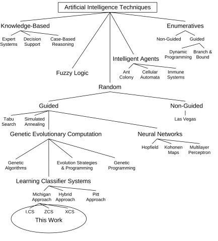
Since the inception of AI research, the increasing availability of computing power, both in institutional form and in the availability of personal computers, has led to a rapid expansion in theory and techniques. This continually changing landscape has resulted in difficulties in defining the exact nature of techniques and families of techniques (DeJong and Spears 1993). Figure II-1, based on work by Alba (Alba and Cotta 1998; Alba 2004) and adapted by Browne (Browne 1999), provides one typology of different AI techniques. As the figure depicts, there are many classes and categories of AI techniques, all slightly different in their approaches to harnessing computing power and the computer’s ability to learn. As shown in Figure II-1, the current research involves a class of techniques which may be considered part of the Genetic Evolutionary family. While the figure depicts LCS-based algorithms and Genetic Algorithms as two distinct families, LCS-based implementations borrow heavily from genetic algorithm-based research.

(31)

Figure II-1 Artificial Intelligence Family Tree

Artificial Intelligence Techniques

Knowledge-Based Fuzzy Logic Intelligent Agents Enumeratives Expert Systems Decision Support Case-Based Reasoning Random Ant Colony Cellular Automata Immune Systems Non-Guided Guided Dynamic Programming Branch & Bound Guided Tabu Search Simulated Annealing Las Vegas Non-Guided Neural Networks Genetic Evolutionary Computation

Hopfield Kohonen Maps Multilayer Perceptron Genetic Algorithms Evolution Strategies & Programming Genetic Programming

Learning Classifier Systems

Michigan Approach Hybrid Approach Pitt Approach

LCS ZCS XCS

This Work

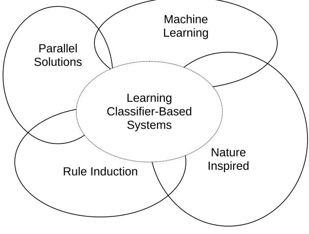
Using a different artificial intelligence typology, LCS and XCS may also be thought to belong to other classes of techniques, drawing inspiration from areas such as Parallel Solutions, Machine Learning, and Nature Inspired (Browne 1999), as depicted in Figure II-2.

(32)

Figure II-2 Classes of Techniques That Contain Learning Classifier Systems

Machine Learning

Nature Inspired Rule Induction

Parallel Solutions

Learning Classifier-Based

Systems

(3) Artificial Intelligence Strategies

Historically, Evolutionary Algorithms used in various AI techniques have consisted of three well-defined paradigms: Evolution Strategies, Evolutionary Programming, and Genetic Algorithms (GA) (Bäck 1996). The first two techniques rely primarily on mutation to evolve, while Genetic Algorithms use recombination to effect adaptation and learning. Moreover, while Evolutionary Programming represents individuals as finite state machines, Evolution Strategies uses real values on a genetic level and Genetic Algorithms use bit strings (Schwefel 1995). As these separate techniques developed and became more mature, however, these distinctions disappeared as beneficial methods from one technique were adopted into others (Goldberg, Deb et al. 1991).

The term Evolutionary Algorithms has now been superseded by Evolutionary Computation (EC), which is also the title of the international journal for the field (DeJong and Spears 1993). Evolutionary Computation recognizes that the boundaries between the techniques are less clear than previously defined, that new techniques are emerging (e.g. Genetic Programming), and that

individual methods are less important than the strategies used when categorizing techniques (Koza 1992).

(33)

(a) Overarching Strategy

The overarching strategy of Evolutionary Algorithms was one of optimization. This was perhaps most apparent in Genetic Algorithms where an entire population was devoted to the

discovery of a single, optimum individual. Although optimization is still a major task in Evolutionary Computation, the single optimum has been augmented by other objectives. Co-adaptation, multiple objectives, and robust optima have all been the subject of algorithmic search (Davis 1991). Genetic Algorithms have been developed that can find local optima as well as locating the global optimum (Goldberg 1989).

Learning Classifier-based systems, the focus of this research, are driven to optimize a

population of rules that are themselves optimum in local niches. This requires the important concept of cooperation for the rules to form a complete optimum. The increase in strategies has led to more problem types becoming solvable through the use of Evolutionary Computation techniques

(Browne 1999).

(b) Representation

Evolutionary Algorithms were tied to the concept of natural systems, so information was generally represented in terms of genotypes (the encoding of parameters) and phenotypes (the response of an individual to an environment). Genetic Algorithms represent knowledge using bit strings, while knowledge encoding in Evolutionary Programs and Expert Systems were typically implemented in a more natural language form (Bäck, Fogel et al. 1997). The representation of most Evolutionary Computation techniques can be a natural form, a bit form, or a domain specific representation. Over time, the flexibility of representation using the traditional ternary (0, 1, #) representation was expanded to include multiple punctuation, logical, and mathematical operators (Koza 1992; Wilson 1999).

(c) Supervision

The three types of supervision that may be applied to a learning technique are summarized by Smith and Dike (Smith and Dike 1995) following on work by Barto (Barto 1990):

1. Supervised learning: the environment contains a teacher that (directly or indirectly) provides the correct response for certain environmental states as a training signal for the learning signal.

2. Unsupervised learning: The learning system has an internally defined teacher with a prescribed goal that does not need utility feedback of any kind.

(34)

3. Reinforcement learning: The environment does not directly indicate what the correct response should have been. Instead, it only provides reward or punishment to indicate the utility of actions that were actually taken by the system. This type of supervision forms the basis of learning in Learning Classifier Systems and is explained in greater detail in the next section.

(4) Machine Learning

The ability to learn is central to Learning Classifier-based machines, so understanding the types of learning used within Artificial Intelligence assists in understanding the current research and its underlying algorithms. Soon after the advent of the electronic computer, scientists envisioned its potential to exhibit learning behavior. Early work by Samuel (Samuel 1959) and others prompted the development of a number of learning machines and different approaches to Machine Learning.

Various authors have used different, but related definitions of learning. The following

definitions are relevant to the present study. Holsapple, Pakath, Jacob, and Zaveri describe human learning “as an amalgam of knowledge acquisition and skill acquisition” (Holsapple, Pakath et al. 1993). Narendra and Thathachar propose the following, behavior-oriented, view: “Learning is the ability of systems to improve their responses based on past experience” (Narendra and Thathachar 1989). Michalski, Carbonell, and Mitchell define learning more cognitively: “Learning processes include the acquisition of new declarative knowledge, the development of motor and cognitive skills through instruction and practice, the organization of new knowledge into general, effective

representations, and the discovery of new facts and theories through observation and

experimentation” (Michalski, Carbonell et al. 1983). A common theme in these definitions is an improvement in the behavior of the system towards an environment, originating from repeated instructions from that environment.

Because this research is specifically concerned with the ability of machines to demonstrate learning behavior, it is also instructive to consider more focused definitions. The following descriptions are particularly relevant to the present study and may be used to indicate whether learning has occurred:

An agent (Machine Learning system) learns (with respect to an environment) if its production of a response alters the state of the environment in such a way that future responses of the same type tend to be better (Kondratoff and Michalski 1990).

(35)

Systems that are capable of making changes to themselves over time with the goal of improving their performance on the tasks confronting them in a particular environment are said to demonstrate learning (Kondratoff and Michalski 1990).

Many different approaches have been used to implement Machine Learning. The specific approach used in a particular research study is often based on the task to be learned, the way in which the task is performed, and on popular theoretical views at the time. For the purposes of this research, Machine Learning will be categorized according to Michalski, Carbonell, and Mitchell’s Machine Learning classification scheme. The classifications, ordered approximately in descending need of required supervision from a teacher are rote learning and direct implementation of new knowledge, learning from instruction, learning by analogy, learning from examples, and learning from observation and discovery (Michalski, Carbonell et al. 1983).

(a) Learning by Rote

Rote learning and direct implementation is the most basic way of learning. It amounts to directly inserting knowledge into a system, either by programming it or by putting the knowledge into a database (Michalski, Carbonell et al. 1983). The system that learns by rote performs no inferencing whatsoever; the emphasis is instead on learning through memorization and the development of indexing schemes to quickly retrieve memorized knowledge when needed (Holsapple, Pakath et al. 1993). The system itself does nothing with the knowledge, except for extracting, executing, storing, and reproducing it (Michalski, Carbonell et al. 1983).

(b) Learning from Instruction

Learning from instruction requires more effort on the system’s part; it is very much like education at school. The learning system must be able to understand, store, and integrate

instructions with what it already knows (Michalski, Carbonell et al. 1983). The system depends on external sources to incrementally present it with knowledge in an appropriately organized form, and then selects new knowledge that must be acquired. It then performs syntactic reformulation of this knowledge to integrate it with existing knowledge (Holsapple, Pakath et al. 1993).

(c) Learning by Analogy

The third category, learning by analogy, requires yet more effort from the system. The system must find in its existing knowledge something similar to the task to be learned and change the knowledge already present until it is applicable to the situation at hand (Michalski, Carbonell et al.

(36)

1983). The system must then store this newly acquired knowledge in its knowledge base until it is ready to be used. Another way to define analogical learning is the retrieval, transformation, and augmentation of relevant existing knowledge into new knowledge that is appropriate for effectively dealing with a new problem that is similar to some previously encountered problem (Holsapple, Pakath et al. 1993).

(d) Learning from Examples

In this type of learning, the system is presented an example from an environment and information to associate with the example. This information can be an indication of whether the example is positive or negative, whether the response of the system was good or bad, or some action to associate with the example. If the information is given at the same time as the example, it is called “true learning with examples” (Michalski, Carbonell et al. 1983). If the information is given after the system has generated a response, it is described as “reinforcement learning” (Kovacs 2002). As will be described later in this chapter, learning classifier-based systems make extensive use of

reinforcement learning; therefore, it is useful to describe this technique in some detail.

A depiction of a general reinforcement learning scheme is provided in the following diagram. As the figure indicates, the system interacts with the environment, receiving inputs and emitting actions that affect the environment and which may result in payoffs.

Figure II-3 General Reinforcement Learning Framework

Environment

Learning System

Reinforcement

Example Response

This framework above represents the key concepts behind reinforcement learning, which has often been chosen as the appropriate framework for developing learning machines that can function autonomously (Wilson 1999). Reinforcement learning is frequently chosen as the learning

mechanism in machines because it is often unclear to a human what a machine must do in order to achieve a defined goal; humans do not “see” the environment the way a machine does, and therefore cannot predict how the machine’s actions will affect the environment. The desired end results, however, are often known and rewards can be attached to them. A programmer might say, for example, “I want the machine to find as much dirt as possible, so I will give the machine a small

(37)

payoff every time it finds some.” This reward mechanism is usually much easier to implement than prescribing exactly what steps the machine must perform to find dirt, as a teacher in a learning instruction environment might do (Wilson 1999).

(e) Learning from Observation and Discovery

The last class of learning, learning from observation and discovery, or unsupervised learning, is the most sophisticated type of learning. In this type of learning, the learning system is left on its own to explore its environment and try to make classifications of phenomena it sees or to form theories about it (Michalski, Carbonell et al. 1983). A system employing this strategy learns by examining a relevant environment that contains one or more concepts of interest without explicit external guidance. The system must then identify, capture, codify, and store relevant concepts from the environment without any supervision (Holsapple, Pakath et al. 1993). Observation may be carried out passively, without disturbing the environment in any way, or through active interaction with the environment.

C. LEARNING CLASSIFIER SYSTEMS

Having now addressed AI and its key components as related to this research, the following sections provide working descriptions of a traditional learning classifier-based system and its more recent variants.

The learning system of interest in this research is called a classifier system. Learning classifier systems (LCS) are a Machine Learning paradigm first posited by Holland in the mid-1970s (Holland 1975), that learns syntactically simple string rules, called classifiers, to guide its performance in an unknown and arbitrary environment. The classifier system derives its name from its ability to “classify” inputs from its environment into sets, and to recommend actions based on those sets. Classifier systems are similar in many respects to more traditional control systems. Just as control systems use feedback to “control” or “adapt” their outputs for particular environments, classifier systems use feedback to “teach” or “adapt” their classifiers to their unique environments (Dorf 1983; Kovacs 1996).

The classifier system has developed from the merging of expert systems and genetic algorithms (Holland 1975; Charniak and McDermott 1985; Waterman 1985). This synthesis has overcome the main drawback to expert systems; namely, the long task of discovering and inputting rules. Using a genetic algorithm, the classifier system autonomously learns the rules needed to perform in a given

(38)

environment. In the current study, this environment is a simulated game of the Iterated Prisoner’s Dilemma.

In Holland’s original work, two ideas emerged which became key topics for future research on Machine Learning. The first idea was that the Darwinian theory of enhanced survival of fitter entities could be used to trigger the adaptation of an artificial system to an unknown environment. This idea later became the basis of research areas like Evolutionary Computation, Adaptive Behavior, and Artificial Life (Lanzi and Riolo 1999). The second revolutionary idea proposed by Holland was that a system could learn to perform a task just by trying to maximize the rewards it received from an unknown environment. This mode of learning through “trial and error”

interactions has been formalized and developed in the area of Reinforcement Learning, which is now a major branch of Machine Learning research (Lanzi and Riolo 1999). Reinforcement Learning, as originally postulated by Holland, is closely related to Michalski, Carbonell, and Mitchell’s Learning by Example classification described in Chapter II: B. (4) (d) . Because most environments are not static and because learning can never be said to be complete, the classifier learning process may never be complete.

(1) LCS-0: A “Traditional” Learning Classifier System

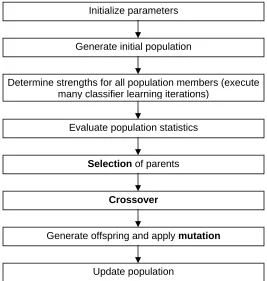
The following sections present a simple classifier system as first described by Holland and Reitman (Holland and Reitman 1978). The significant components of the classifier system are described, including the genetic algorithm (GA). Because the GA plays a vital role in the classifier system’s learning ability, the major aspects of this algorithm are examined in some detail. After the introductory explanation of the classifier system’s components, the entire learning classifier system is presented, depicting the interaction of its various components. After exposition of the classifier system and the genetic algorithm, a number of exemplar learning classifier system applications are reviewed.

(a) LCS-0 Architecture

A classifier system has three major components: • Rule and message subsystem,

• Apportionment of credit subsystem, and

• Classifier discovery mechanisms (primarily the genetic algorithm).

Figure II-4 depicts how the classifier system interacts with its environment. As described previously in Chapter II: B. (4) (d) and illustrated in Figure II-3, classifier systems behave according

(39)

to the mechanism employed in “Learning From Examples.” The classifier system receives

information about the environment, performs internal processing and then affects the environment. It then uses feedback about the effect on the environment to learn from the experience. Figure II-4 shows the classifier system in learning mode, because the classifier system is using the feedback to learn from experience. Conversely, if no feedback is provided, the classifier system is said to be in application mode. Application mode is used after sufficient learning has been accomplished. The following discussion, up until Chapter II: C. (1) (d) Classifier Systems: The Holistic Viewpoint deals with the classifier system exclusively in learning mode.

Figure II-4 Interactions between Classifier System and Environment Environment

Learning Classifier System

Payoffs/Feedback

Inputs Actions

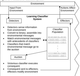
Figure II-5, Traditional Learning Classifier System Modules provides more detail on the classifier system’s internal components. In Figure II-5, the Detectors, Effectors, and Classifier Population blocks make up the rule and message subsystem; the Auction and Reward/Punishment blocks represent the apportionment of credit subsystem; and the Classifier Discovery block signifies the system’s

classifier discovery subsystem. The following subsections describe these components in detail, and provide more information about the information flow between them.

(40)

Figure II-5 Traditional Learning Classifier System Modules

Learning Classifier System

Environment

Payoffs/Feedback

Inputs Actions Detectors Effectors

Reward/ Punishment

Auction Classifier

Population Classifier

Discovery (GA)

Rule and Message Subsystem

Apportionment of Credit Subsystem

Classifier Discovery Subsystem

i. Rule and Message Subsystem

Each classifier consists of a rule or conditional statement whose constituents are words drawn from the ternary alphabet (0, 1, #). The benefit of such a representation scheme is that, just as text is stored on computer disks as 0s and 1s, any rule can be translated into 0s, 1s, and #s, so that it is in the form of a classifier. Once translated, rules can be manipulated more easily, and rule discovery and modification can occur. The alphabet is explicitly restricted to allow for the power of genetic algorithms to be applied to the rule set as described in Chapter II: C. (1) (b) Genetic Algorithm. The alphabet in no way restricts the representational capacity of the classifiers.

Each classifier has one or more words or conditions as the antecedent, an action statement as the consequent, and an associated strength. To illustrate, Table II-1, Samples of Valid Classifiers shows samples of strings that are valid forms for classifiers, (with the “:” symbol denoting the break between the antecedent and action, (i.e. <antecedent>:<action>), in the first column, and their associated strength in the second column.

(41)

Table II-1 Samples of Valid Classifiers

Rule Strength 011:101 23.2

011001##10#110:11 17.3 10101000110011##100#:11100001 32.9

####:1 7.1

The “#” symbol in the ternary alphabet acts as a wild card or “don’t care” in the condition, matching either a 0 or 1. This allows for more general rules; the more “don’t care” symbols, the more general the rule. The measure used to quantify this characteristic is called specificity. The specificity of a classifier is the number of non-# symbols in the antecedent. If a classifier’s

antecedent consists of all # characters then the specificity is zero; if there are no # characters in the antecedent then the specificity is equal to the antecedent’s string length.

The messages, generated either from the environment or from the action of other classifiers, match the condition part of a classifier. Therefore, an action is a type of message, with the consequence of an action being the modification of the environment (or the attempted matching with another classifier in some classifier systems). In this study, classifiers only match messages from the environment and actions generated from classifiers only affect the environment.

For a condition to match a message, every part of the condition string must match every part of the message string. Therefore the message,

011001

would match all of the following conditions 0110#1

011001 ##100# ###### as well as others.

The strength of a classifier provides a measure of the rule’s past performance in the environment in which it is learning. That is, the higher a classifier’s strength the better it has

performed and the more likely it will actually be used when the condition matches an environmental message (refer to Chapter II: C. (1) (a) ii. a. for details) and to reproduce when the GA is applied (refer to Chapter II: C. (1) (b) for additional information). The strength values are relative; therefore, a range limit is set. If the classifier strength falls out of this range, the strength value can be set to the closest range extreme to eliminate the range violation.

The rule portion of a classifier has the template:

(42)

IF <condition> THEN <action> where

<condition> is encoded as a string from the alphabet, and

<action> is also encoded as a string from the alphabet.

This form differs from those normally found in expert systems. In expert systems, the rules often consist of sentences, for example:

IF the patient exhibits symptom X, THEN diagnose illness Y

As opposed to the classifier system’s ternary alphabet representation, such syntax makes it very difficult for a computer system to be able to modify such a rule.

The messages from the environment are filtered and converted via input sensors. The sensors (called detectors in classifier system parlance) discriminately select certain aspects of the

environment to sense and then translate the input to a binary form which can be processed by the classifiers.

The actions of matching classifiers modify the environment via the effectors (or output

interface) as depicted previously in Figure II-5, Traditional Learning Classifier System Modules. The effectors translate the binary action into a form which is appropriate to modify the environment within an envelope of allowable modifications.

ii. Apportionment of Credit Subsystem

The apportionment of credit subsystem deals with the adjustment of the strength of classifiers as the classifier system learns (Booker, Goldberg et al. 1989). In a traditional LCS, strength

adjustments occur via three interrelated mechanisms: • Auction,

• Reinforcement and punishment, • Taxation.

As the classifier system receives messages from the environment, all the classifiers that match one (or more) of the messages compete, by submitting a bid, in an auction to determine a victorious classifier that will affect the environment. Chapter II: C. (1) (a) ii. a. further discusses the auction. The victorious classifier’s effect will be beneficial or detrimental to the environment. With this feedback, the apportionment of credit subsystem appropriately uses reinforcement and punishment to increase or decrease the strength of the victorious classifier that modified the environment. Chapter II: C. (1) (a) ii. b. Reinforcement and Punishment details how feedback from the

(43)

environment is used with reinforcement and punishment. Finally, taxation is levied on each classifier per iteration and on each classifier that submits a bid during an auction. Details of and the need for taxation are provided in Chapter II: C. (1) (a) ii. c. Taxes.

Computer simulations show that the exact mechanism for the apportionment of credit subsystem is not critical to the learning ability of the classifier system (Riolo 1988). That is, the apportionment of credit subsystem may have many forms and the classifier system will still learn, albeit incrementally more efficiently with the apportionment of credit subsystem in some forms than others. This is an example of one of the many classifier system parameters which may vary in

different classifier system implementations. The values to which the parameters should be set to cover a range, guided by biological analogy and empirical results. Many times the parameters are manipulated during the learning process to determine if such manipulations can enhance learning (Riolo 1988).

a. Auction: Bidding and Competition

An auction is performed among all the classifiers that have an antecedent that matches at least one of the environmental messages. The classifier system’s detectors receive input from the

environment and assemble the input into environmental messages. Each classifier attempts to match each environmental message, with each classifier that matches bidding in the auction.

With the matching classifier pool determined, the auction commences. Each classifier participating in the auction submits a bid; the bid is a function of the classifier’s strength and specificity. Only the bid of the victorious classifier is paid, so only the victorious classifier has its strength decreased by the amount of its winning bid. The bid of classifier i at iteration t, B_i(t), is calculated as:

Equation II-I Calculation of Classifier’s Bid

(t) i S * ) BRPow BidRatio *

2 k 1 (k * 0 k (t) i

B = +

where

(44)

Table II-2 Classifier Bid Variables Parameter Description

k0 Classifier Bid Coefficient: positive constant less than

one that acts as an overall risk factor influencing what proportion of a classifier’s strength will be bid and possibly lost on a single step.

k1 Bid Coefficient 1: constant less than one for

non-specificity portion of bid.

k2 Bid Coefficient 2: constant less than one for

specificity portion of bid.

BidRatio Measure of the classifier’s normalized specificity. A BidRatio of 1 means there is just one possible message that matches its condition, while a BidRatio of zero means the classifier would be matched by any message and the antecedent would consist of all wildcard characters.

BRPow Parameter controlling the importance of the BidRatio in determining a classifier’s bid (default is 1).

Si(t) Strength of classifier i at step t.

Figure II-6, shown on the next page, provides a simplified view of how the auction functions.