Empirical Evidence on the North South Trade Flows: an Augmented Gravity Model

(1)

Munich Personal RePEc Archive

Empirical Evidence on the North-South

Trade Flows: an Augmented Gravity

Model

Giorgio, Ricchiuti

Dipartimento di Scienze Economiche, Università degli Studi di

Firenze

2004

Online at

https://mpra.ub.uni-muenchen.de/1326/

(2)

Empirical Evidence on the North-South

Trade Flows: an Augmented Gravity

Model

Giorgio Ricchiuti, University of Florence

1

April 2004

[email protected]

Abstract

In this paper we analyse the determinants of the trade flows between Developed

and Developing Countries using an augmented version of the Gravity Equation.

We add two extra variables: the technological distance and the bilateral real

exchange rate (RER). The former allows us to analyse the impact of the

technological gap on trade structure, the latter to study the movement in the

relative prices and their impact on trade pattern. We estimate a Fixed Effects

Model (FEM) for different groups of countries. The sign and the numerical value

of the coefficients of GDP and Population are different when we analyse

separately emerging countries as importers or exporters. This result supports the

assumption that determinants of trade, for the two areas (Developed vs Emerging

Countries), are not the same. Moreover, as expected, the geographical and the

technological distance appear as barriers to trade, and the positive effect on

export of a devaluation of the bilateral real exchange rate is confirmed by our

results.

1_{I am grateful to Vasco Molini, Carlo Filippini and Dario Pozzoli who allowed me to use their}

(3)

Introduction

In the last two decades, partly due to enhancements in statistical analysis, both

empirical and theoretical articles have improved the Gravity Theory. Very

different problems, such as flows of migration, FDI and trade, have been

analysed making use of the Newton’s Law:

2

ij J i

ij

M

D

GF

=

where

i

≠ j (1)

the gravitational attraction of two bodies (GF) is directly proportional to their

Mass (M) and indirectly proportional to their Distance (D).

After the Second World War, the growth in the international trade flows boosted

the number of empirical studies trying to analyse the determinants of the trade

pattern. Timbergen [1962] and Linnemann [1966] have been the first authors to

transfer the Gravity Equation (1) to the empirical analysis of international trade

flows. In their first formulation, they related trade between countries to the mass

of the economic system (proxied by GDP) and to the physical distance between

them (as proxy of the transaction costs). Even if the formulation was

parsimonious and empirically robust, initially the Gravity Analysis lacked a

strong theoretical background.

It is only after the pioneering work of Anderson [1979] that many authors either

have tried to lead the gravity equation to a formal economic theory (i.e.

Bergstrand [1985,1989], Helpman and Krugman [1985]) or have discuss the

implication of the gravity equation in a neoclassical world (Deardoff, 1995)

In this paper the Gravity equation is used to analyse the trade flows between

North (11 European countries, USA and Japan) and Emerging Countries (5

south-east Asian and 6 Latin American countries) in the last two decades (from

the 1980 to the 2000).

In the line of Egger [2000,2002] and Matyas [1997,1998] the analysis is

carried out by a panel framework, which enable us to take into account the

connection between the explanatory variables over a long period, to reduce the

(4)

and to identify the country (in our case the bilateral) specific effects [Green

1997].

In order to develop a more precise analysis, different panel dataset have been

built. The underlying assumption is that, to clarify how different variables affect

the trade pattern, developed and developing countries have to be split. Moreover,

the flows of manufacturing and non-manufacturing goods have to be investigated

separately, to highlight the impact of different explanatory variables. For

instance, given a strongest price competition on these markets, a bigger effect of

a variation of the real exchange rate could be expected for the

non-manufacturing goods.

The analysis is therefore developed for four dataset, i.e. the combination of the

manufacturing and non-manufacturing goods, and bilateral trade flows from

developed (exporters) to developing (importers) countries.

The first section describes the model and explains how the real exchange rate

(thereafter rer) and technological distance (techdist) have been built. Section 2

develops the correct econometric specification of the model. Section 3 reports the

results for each dataset. Finally, in section 4, we draw some conclusions and

provide suggestions for further analysis.

The Augmented Model

According to the above Newton’s Law, basic Gravity equation for trade flows

may be written as follows:

ijt jt it ijt

osts TransportC

Y AY

TradeFlow = (2)

where

it it it

Population GDP

Y =

jt jt jt

Population

GDP

Y

=

.

(5)

The GDP per capita is used as proxy for the Mass of the two bodies (countries

in our case) and transport costs are the proxy for Distance (A is a constant of

proportionality). Although this specification is the most employed, we have

preferred to analyse separately the impact of GDP and population on imports, to

stress their differences. Moreover, differently from this equation, the trade flows

here analysed are the imports of country i.

Even if the transport costs could be model more precisely using proxies (i.e.

infrastructure, the price of fuel, physical shipping costs) the geographical

distance among the two countries has been typically used as a proxy.

In this paper we add rer (bilateral real exchange rate) and distec (bilateral

technological distance) to the standard specification to capture how the

movement in the relative prices and the exchange rate affect the trade pattern

and how the technological gap can influence the trade structure.

The logarithmic form for the estimated equation is as follows2_:

ijt t ij ijt ji ij jt it jt it ijt ijt

u

techdist

rer

ce

dis

gdp

pop

imports

ε

λ

β

+

=

₋ 8 7 6 5 4 3 2 1 1 0

tan

(3) where: ijt

imports

the imports of the country i from the country j at the time t.

0

β

the constant

it

pop

the population of the country i at time t

jt

pop

the population of the country j at time t

it

gdp

the GDP of the country i at time t

jt

gdp

the GDP of the country j at time t

ij

ce

dis

tan

the geographical distance among country i and country j

ji

rer

the bilateral real exchange rate of the export country, see below for the

construction

ijt

distec

technological distance among the country i and the country j

ij

u

fixed country-pair effects

2_{In the regressions the lagged dependent variable is introduced. It will be explained in the}

(6)

t

λ

time (business cycle) effects t=1....T

ijt

ε

normal error terms with mean zero and variance

σ

_ε2.

To catch the possible differences in trade pattern among Latin American and

Southeast Asian countries, we introduce a dummy variable ‘la’ (equal 1 for Latin

American countries, 0 otherwise).

The Real Exchange Rate

As suggested by Matyas [1997], the bilateral real exchange rate can affect trade

flows. In this paper, a huge difference between Latin American and Southeast

Asian countries is expected: the volatility of both exchange rate and prices in LA

is likely to be the major cause of a reduction in the trade flows. As stated above,

this effect will be analysed using the dummy la.

The real exchange rate can be defined as the ratio of the price level of the

typical basket of goods and services in country 1 to country 2. Following

Edwards [2000]:

j i i j i j

P

E

RER

_,

=

,

*

(4)

where, E is the bilateral nominal exchange rate, P* a price index of the foreign

country and P is a domestic price index (i is the importer and j the exporter). The

SDR (the unit of account of the International Monetary Fund) has been used to

achieve the bilateral nominal exchange rate3_:

i j

Currency

SDR

Currency

E

_,

=

*

(5)

The Producer Price Index4_{(PPI) of the importer has been used as proxy for}

traded goods prices and the Consumer Price Index of the exporter for the

domestic price index.

(7)

Finally, to compare data, the variable has been convert in US dollar, by

multiplying the equation (4) by the bilateral nominal exchange rate US dollar per

national (Exporter) currency. Hence, our variable is:

i US i

j j i USD

j

i

E

CPI

PPI

E

RER

_,

=

,

(

)

_, (6)

To separate the cyclical behaviour of the RER, we apply the Hodrick-Prescott

filter5_{. Moreover, to catch a lagged effect of a}_real_{devaluation, the effect of the}

lagged RER has been examined.

We expect a positive sign for RER: devaluation (i.e. a rise of the variable) should

imply an increase of the imports of country i. Moreover, as pointed out above, a

larger coefficient (in absolute value) is expected in the regression investigating

non-manufacturing trade flows.

The Technological Distance

6

Differently from the Newtonian concept of Distance, in social sciences the

Distance between two Masses may be not only geographical but also due to both

cultural and historical differences and those one in the structure of the economic

system. Filippini et al. [2003] have tried to explore the latter; building a variable

to capture the technological distance to study this kind of Distance among

Developed and Emerging countries has an effect on the trade pattern. The sign of

the constructed variable may help to understand whether the gap reduces the

flows or it may be a flywheel for trading [ibid.]. Hence, it can be negative or

positive. As shown below, in we find a significant negative sign of coefficient,

confirming that the more the countries are “technologically” close, the more they

trade.

The variable techdist is defined as the absolute difference between the

technological indicators (TI) of the two trade partners.

5_{See the classical article of Hodrick and Prescott [1981] or, for a basic analysis Ahumada and}

Garegnani [1999]

6_{For a more exhaustive definition and discussion on how this variable affect the trade flows see}

(8)

distecijt =

TI

it

−

TI

jt (7)

The TI indicator is a simple average of three different dimensions: creation of

technology, diffusion of technology and human skills.

The Balassa’s Relative Comparative Advantage Index (Balassa 1965) in Medium

and High Tech sectors (HMTRCA) is used as proxy for creation of technology,

HMTRCAit =

wt wt it it EXPtot EXPmht EXPtot EXPmht (8) where:

• EXPmhtit = the medium/high-tech exports of country i at t-time.

• EXPtotit = the total exports of country i at t-time.

• EXPmhtwt = the world medium/high-tech exports at t-time.

• EXPtotwt = the world total exports at t-time.

Diffusion of technology is computed as a simple average of electricity

consumption, telephone penetration and internet users (since 1994).

And finally, the average of secondary and tertiary enrolment ratios plus the

literacy rate has been employed to work out a proxy of human resources.

The following general formula (9) has been utilised to express the second and

third indexes in an interval [0,1]; the maximum and minimum values are

respectively the USA’s and the zero:

it

Index

x =

t t t it

value

Minimum

value

Maximum

value

Minimum

value

Actual

−

(9)

Hence, the overall Technological Index for country i at the time t is:

3

skills it diffusion it it it

Index

HMTRCA

(9)

The Econometric Specification

As Matyas [1997] pointed out, the traditional cross-section or time-series

approaches are affected by a severe problem of misspecification, when used to

study the Gravity Equation. Indeed, the equation (3) as a generic form of all

econometric specification used to analyse the Gravity Equation [Matyas 1997]. A

cross-section analysis implicitly assumes T=1 and

λ

_t

=

0

. On the other hand Time series analysis assumes

u

_ij

=

0

. This leads, as suggested by Egger [2000] and Matyas [1997], to properly specify the Gravity Equation by a triple index panel

model7_{(a two way error component regression model), which does not present}

such a kind of restrictions [Baltagi 1995]. Table 18_{shows that not including}

these effects may lead to incorrect inference.

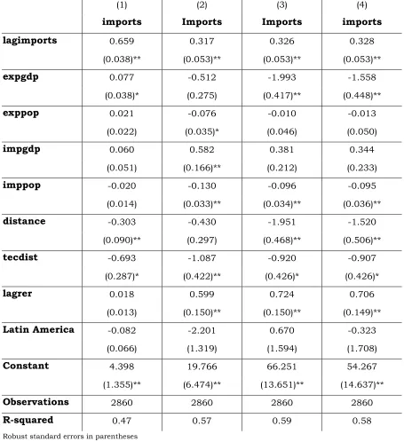
Let us compare results reported in Table 1. Regression (1) is a simple OLS,

without any time or country-pairs effects, regression (2) is a one-way error

component model (where

λ

t

=

0

is assumed), while9 regression (3) is our

preferred specification, with both time and country-pairs effects. Differences

among regression (1) and (2)-(3) are large: both the absolute value of the

coefficients and the signs are different. More precisely, the signs of the exporter’s

GDP and Population switch (from positive to negative). Moreover, the coefficients

of variables in regressions (2)-(3) are larger than those one in the regression (1),

except for the lagged of imports (which is the half). Finally, the significance of

some coefficients is quite different.

On the other hand the comparison of regression (2) and (3) leads to different

results. With the exception of the dummy LA, the signs and the size of the

coefficients are the same. However, the exporter’s GDP and the geographical

distance, insignificant for the regression (2), are significant for the regression (3).

On the other hand, exporter’s population and importer’s GDP are not significant

in the regression (3), even if exporter GDP is significant at 10 % of confidence

level.

7_{In our analysis it is transformed in a double-indexed model, since we use a country-pair effect.} 8_{For parsimony we prefer to show this result just for the first dataset: trade flows from developed}

(exporters) to emerging (importers) countries. Moreover, the coefficients of both time and country-pair effects have been excluded

(10)

[image:10.595.82.537.120.618.2]

Table 1- Comparison among different Specification

(1) (2) (3) (4)

imports Imports Imports imports

lagimports 0.659 0.317 0.326 0.328

(0.038)** (0.053)** (0.053)** (0.053)**

expgdp 0.077 -0.512 -1.993 -1.558

(0.038)* (0.275) (0.417)** (0.448)**

exppop 0.021 -0.076 -0.010 -0.013

(0.022) (0.035)* (0.046) (0.050)

impgdp 0.060 0.582 0.381 0.344

(0.051) (0.166)** (0.212) (0.233)

imppop -0.020 -0.130 -0.096 -0.095

(0.014) (0.033)** (0.034)** (0.036)**

distance -0.303 -0.430 -1.951 -1.520

(0.090)** (0.297) (0.468)** (0.506)**

tecdist -0.693 -1.087 -0.920 -0.907

(0.287)* (0.422)** (0.426)* (0.426)*

lagrer 0.018 0.599 0.724 0.706

(0.013) (0.150)** (0.150)** (0.149)**

Latin America -0.082 -2.201 0.670 -0.323

(0.066) (1.319) (1.594) (1.708)

Constant 4.398 19.766 66.251 54.267

(1.355)** (6.474)** (13.651)** (14.637)**

Observations 2860 2860 2860 2860

R-squared 0.47 0.57 0.59 0.58

Robust standard errors in parentheses

* significant at 5% level; ** significant at 1% level

(1) OLS with _u_ij=₀and λ_t =0

(2) one-way error component model: ₌₀ t

λ

(3) two-way error component model

(4) IV using lags of the most likely endogenous independent variables

There is another problem which we have to deal with to achieve a proper

(11)

for example, that the imports and the GDP at time t are implicitly related. The

existence of not strictly exogenous variables may lead to simultaneous bias. As

Matyas [1997, 1998] suggests, we can by-pass this problem using the lags of the

most likely endogenous independent variables as their instruments. Regression

(4) shows that except from the dummy La, for which the sign of the coefficient

change (even if it is not significant), IV model has the same sign and similar

numerical values than model (3), suggesting that in our case simultaneous bias

is not a severe problem. Hence, we will report in our analysis the regressions not

instrumented.

Finally, we have to discuss how to treat the country-pairs effects has to be

managing and how to work out the time-invariant variables in a fixed effect

model.

Since the individual (country-pairs) effects (

u

ij) have been included in the

model, we have to decide whether they are considered as fixed or random. From

an econometric point of view the problem could be solved by the Hausman test

[Green 1997]. Nevertheless, this test may not be unidirectional when more

regressions are run. As Hsiao [1995] and Matyas and Harris [1998] pointed out,

if the statistics are not fully conclusive, the objectives of the study should be

considered. Given that the purpose of this paper is to analyse the trade flows

between a predetermined selections of countries [Egger 2000], the FEM seems

consistent with the model. Nevertheless, it is worth noting that, “the random

effect model may be preferred as it lends itself to a dynamic specification, of

which the lagged dependent variable is likely to be highly significant” [Matyas

and Harris 1998].

The last problem faced is how achieve the coefficients of the Time-Invariant

variables (geographical distance and la) with the specification assumed. We can

work out the coefficients either estimated an LSDV model or, as we do, using a

Fixed Effect Model, with a second step estimation, retained the fixed values from

the general regression and regressing (with OLS) the time-invariant variables on

those one:

ij ij ij

LA

Lndis

(12)

Where FE are the fixed effects and

ε

_ij are the white noise residuals.

The Main Results

In the econometric analysis we examine 143 trade routes among 13 North

countries (11 European countries, USA and Japan) and 11 Emerging Countries

(5 south-east Asian and 6 Latin American countries) have been recreated over a

period of 21 years (1980-2000). Following the results for each dataset are

discussed. It is worth to briefly discuss the expected signs. First, assuming the

presence of an inertial effect, we expect a positive and significant effect of past

imports. As mentioned above, GDP and Population are analysed separately, since

a different dynamic of the population growth is assumed among Developed and

Emerging Countries. As our primary explanatory variable for the Mass a positive

sign for the coefficient of the GDP is expected: the larger we are the more we

trade. The signs for population’s coefficients may be different in developing or

developed country. In Developed Countries the population is stable and is

therefore not likely to affect the import/export relationship, hence we do not

expect a positive effect. On the other hand, given that the developing countries

are at different stage of the demographic transition, we suppose a strong

influence of population on imports, the sign, however, is not clear. We may have

an import substitution effect. Unfortunately the negative sign could also depend

on the correlation among GDP and Population: given the GDP’s level, the growth

of the population causes a reduction in the income per capita and a consequent

decrease of the imports. We may have a market effect, since a growing population

may need more differentiated (imported) goods.

The Newtonian distance is performed by both geographical and technological

distance. We expect a negative coefficient for both. However, while for the former

a negative relation is realistic, for the latter, as stated above, the sign could be

ambiguous.

Different is the assumption about the bilateral RER of the exporter country. A

real devaluation for country j has a positive effect on imports of country i.

Nevertheless, we use the lagged RER: devaluation now will show its effect next

(13)

Finally, assuming that there has been a swap between Latina America and East

Asia in the commercial relationship with the Developed Countries a negative sign

of the Dummy LA is expected.

Flows From Developed (exporters) to Emerging (importers)

Countries

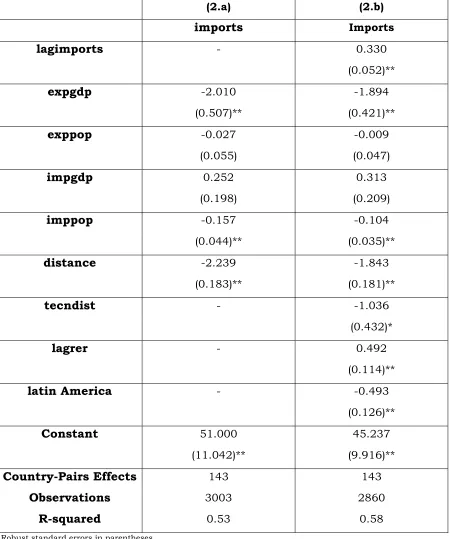
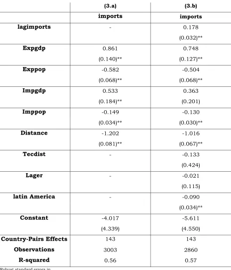
Table 2 and Table 3 show our preferred regressions: respectively the basic and

the augmented gravity. The dependent variable is imports of Emerging Countries

for either manufacturing (Table 2) or non-manufacturing (Table 3) goods.

In Table 2, all variables, except for exporter’s population and importer’s GDP,

are significant at 5%. However, the sign of some coefficients is different from

expected.

Indeed, the signs of both GDP variables were expected positive, being our mass

variable.This is true only for the importing country but not for the exporting one.

The counterintuitive result may depend on the aggregation level of our data: a

strong sector-based effect could be leading the negative sign. Moreover we are

virtually looking at two blocks, developed versus emerging countries, excluding

the possibility of the intra-blocks trade. Finally, there may be negative effect of

the variable techdist on GDP, which compensate the mass positive effect of the

GDP on imports, cancelling each other out.

The signs for the population variables are both negative (2.a and 2.b), even if

the exporter’s one is not significant. As stated above, it may indicate an

import-substitution effect: the bigger the population the larger the production for the

domestic market.

Both geographical and technological distances show a negative coefficient.

Particularly, the latter, as pointed out above, highlights how a technological gap

is an obstacle to trade. Moreover, its absolute value is bigger for manufactured

goods (2.b) than for non-manufactured one (3.b).

For manufactured goods the real exchange rate lagged clearly affects trade

flows: depreciation (for the country j) of the real exchange rate at time t-1 implies

(14)

[image:14.595.87.537.91.630.2]

Table 2 From Developed to Emerging Countries – Manufactured Goods

(2.a) (2.b)

imports

Imports

lagimports

- 0.330

(0.052)**

expgdp

-2.010 -1.894

(0.507)** (0.421)**

exppop

-0.027 -0.009

(0.055) (0.047)

impgdp

0.252 0.313

(0.198) (0.209)

imppop

-0.157 -0.104

(0.044)** (0.035)**

distance

-2.239 -1.843

(0.183)** (0.181)**

tecndist

- -1.036

(0.432)*

lagrer

- 0.492

(0.114)**

latin America

- -0.493

(0.126)**

Constant

51.000 45.237

(11.042)** (9.916)**

Country-Pairs Effects

143 143

Observations

3003 2860

R-squared

0.53 0.58

Robust standard errors in parentheses * significant at 5%; ** significant at 1%

Finally, the Latin American dummy variable is negative and significant too,

suggesting how the Latinos had lower propensity to trade with the Developed

(15)

[image:15.595.88.553.86.630.2]

Table 3From Developed to Developing Countries - Non Manufactured Goods

(3.a) (3.b)

imports

imports

lagimports

- 0.178

(0.032)**

Expgdp

0.861 0.748

(0.140)** (0.127)**

Exppop

-0.582 -0.504

(0.068)** (0.068)**

Impgdp

0.533 0.363

(0.184)** (0.201)

Imppop

-0.149 -0.130

(0.034)** (0.030)**

Distance

-1.202 -1.016

(0.081)** (0.067)**

Tecdist

- -0.133

(0.424)

Lager

- -0.021

(0.115)

latin America

- -0.090

(0.034)**

Constant

-4.017 -5.611

(4.339) (4.550)

Country-Pairs Effects

143 143

Observations

3003 2860

R-squared

0.56 0.57

* significant at 5%; ** significant at 1%

Table3 (non-manufacturing) presents a roughly different story; It is worth

(16)

countries are small. The sign of GDP variables are both positive, even though the

one of the import country is insignificant for the augmented specification10_.

The coefficients for population (3.a and 3.b) are negative and significant. Even

in this case we may assume a substitution effect; while the importer try to

increase the productivity of the non-manufactured production, the exporter

reduces its export to compensate the increase of the population.

Moreover, as for manufactured goods, the geographical distance and the

technological distance have the expected sign, even though the latter is not

significant. This last result is not surprising, since we believe that technological

distance have a bigger effect on the manufacture.

Contrary on our expectation, moreover, the real exchange rate does have a

negative (even not significant) effect (3.b). As pointed out above, the

non-manufactured goods that the Emerging Countries import from the Developed one

are very small. Hence, such a kind of trade may not depend on the price level.

Finally, the dummy variable for Latin America is again negative, showing the

decreasing of the imports of these countries from the Developed ones.

Flows From Emerging (exporters) to Developed (importers)

Countries

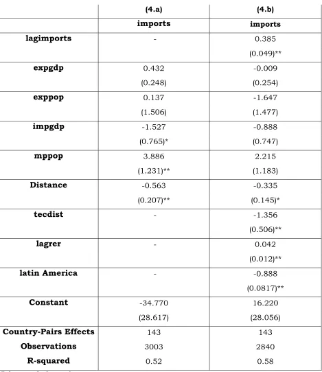
Table 4 and Table 5 report the results of regressions where the dependent

variable is imports of, respectively, manufactured and non-manufactured goods

of Developed Countries.

These two dataset are the counterpart of those reported above11_{. Even if it could}

be argued that the imports of the non-manufactured goods from developed

countries are small (Table 3), it can be noted that in comparison with the Table

2, while the GDP’s coefficients present the same sign and roughly similar

absolute value (Table 2 vs. Table 4 and Table 3 vs. Table 5), those of Population

are completely different. This supports the assumption that developed and

developing countries have to be split.

10

However, this coefficient is significant at 10% level. For parsimony, we have avoided to include the variable significant at 10%.

(17)

[image:17.595.86.555.86.628.2]

Table 4 from Developing to Developed - Manufactured Goods

(4.a) (4.b)

imports

imports

lagimports

- 0.385

(0.049)**

expgdp

0.432 -0.009

(0.248) (0.254)

exppop

0.137 -1.647

(1.506) (1.477)

impgdp

-1.527 -0.888

(0.765)* (0.747)

mppop

3.886 2.215

(1.231)** (1.183)

Distance

-0.563 -0.335

(0.207)** (0.145)*

tecdist

- -1.356

(0.506)**

lagrer

- 0.042

(0.012)**

latin America

- -0.888

(0.0817)**

Constant

-34.770 16.220

(28.617) (28.056)

Country-Pairs Effects

143 143

Observations

3003 2840

R-squared

0.52 0.58

Robust standard errors in

parentheses

* significant at 5%; ** significant

(18)

[image:18.595.82.562.84.635.2]

Table 5 From Developing to Developed Countries - Non Manufactured Goods

(5.a) (5.b)

imports

imports

lagimports

- 0.334

(0.047)**

expgdp

-0.331 0.032

(0.219) (0.290)

exppop

0.810 1.383

(1.162) (1.229)

impgdp

-1.974 -1.793

(0.637)** (0.601)**

imppop

4.016 3.579

(1.064)** (0.989)**

distance

-0.827 -0.432

(0.168)** (0.130)**

tecdist

- -0.175

(0.493)

lagrer

- -0.030

(0.014)*

latin America

- 0.183

(0.091)*

Constant

-27.730 -43.947

(22.929) (25.973)

Country-Pairs Effects

143 143

Observations

3003 2838

R-squared

0.54 0.59

* significant at 5%; ** significant at 1%

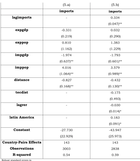
It is worth noting, in both Table 4 and 5, that Exporter’s GDP and Population

(even if they are not significant) change sign12_{when we use the second}

specification (4.b and 5.b). This may confirm the presence of a strong

(19)

multicollinearity among these variables and both technological distance and rer.

The coefficient of the exporter’s (the emerging countries) GDP is close to zero,

suggesting –as pointed out above- an offsetting effect (i.e a negative effect of

techdist against the mass positive effect). On the other hand, in the augmented

specification, the exporter’s population as a huge negative effect in Table 4 and a

positive one in Table 5; however we could expect a different sign when we look at

the typology of goods: an increase in emerging countries population should

decreases (and not increases) their export of non-manufactured goods to supply

the domestic market.

Even for the developed countries, there is a very strong market size effect: a

small increase of the population leads to a huge increase in imports.

The effect of lagged trade is, as always, significant and the numerical value is

large in absolute level. The negative coefficients of both distance variables are

confirmed for both the tables. Again the technological distance is not significant

for the non-manufactured dataset and its absolute value is larger in Table 4 than

in Table 5.

As above, surprising the rer is positive only for the manufactured goods. Finally,

while for manufactured goods the Latin American dummy is still negative; in

Table 5 it is positive and significant. This may suggest that during the period

analysed imports of developed countries from Latin Americans has been

decreasing for manufactured goods but increasing for non-manufactures:

Developed Countries imports manufactured goods from Asian countries and

non-manufacturing from Latin Americans.

Conclusions and Issues

In this paper we have analysed an augmented gravity model, using a triple

index Fixed Effect Model to take into account the bilateral specific and time

effects. Two variables have been added to the basic gravity equation used in the

literature: technological distance and bilateral real exchange rate. Besides, to

capture the differences between Latin America and Southeast Asia, a dummy

variable have been introduced. As expected, analysing separately first the

(20)

the sign and the size of the coefficients of GDP and Population are quite different,

supporting the assumption that the determinants of trade, for the two areas

(Developed vs. Emerging Countries) are not the same. Furthermore, the

geographical and the technological distance outline barriers to trade. Finally,

expected the positive effect on export of the devaluation of the bilateral real

exchange rate is confirmed by data just for the manufactured goods.

In spite of the using of IV regression to look at the simultaneous bias effect,

there are some econometric issues which may have affected our analyses:

a) Lagged dependent variable: from the theory we assume that imports at

time t are highly linked with those one at time t-1, suggesting that

introducing a lagged dependent variable, the dynamic of the relation could

be explained better. However, as pointed out in Matyas and Harris [1998]

the choice between static and dynamic models is not obvious, the

modelling is different and a well-defined procedure does not exist.

b) FEM vs. REM: as argued above the choice between these two models may

not be simple, and does not depend just on the Hausmann test result. For

example, Matyas and Harris [ibid.] suggest that “for strictly more policy

reasons, the random effect model may be preferred, as the effects of

explanatory variables are not diminished the presence of a relatively large

set of dummy variables”.

c) As Egger [2002] pointed out, while the FE (and RE consistent) model

reflect short-run parameters, the Between Effects Model is nearer to

long-run parameters.

Hence, the indication for further analysis is employing a dynamic model (i.e

Arellano Bond model) analysing the differences respect ours; studying the panel

stationary of the real exchange rate and last but not least examining long vs.

(21)

References

Ahumada, H. − Garegnani, M. (1999), “Hodrick-Prescott Filter in Practice”,

mimeo

Anderson, J.E. (1979), “A Theoretical Foundation for the Gravity Equation”, The

American Economic Review, vol. 63, pp.106-116

Balassa, B. (1965), “Comparative Advantages in Manufactured Goods: A

Reappraisal”, Review of Economics and Statistics 168, pp. 315-319

Bergstrand, J.H. (1985), “The Gravity equation in International trade: some

microeconomic foundations and empirical evidence”, Review of economic and

statistics, vol. 67, pp.

Bergstrand, J.H. (1989), “The generalised gravity equation, monopolistic

competition, and the factor-proportions theory in international trade”, The

Review of Economics and Statistics 67, pp. 474-481

Deardoff, A.V. (1995), “Determinants of bilateral trade: does gravity work in a

neoclassic world?”, NBER Working Paper 5377

Edwards, S. (2000), Capital Flows and The Emerging Economies, The University of

Chicago Press

Egger, P. (2000), “A note on the proper econometric specification of Gravity

equation”,Economic Letters, vol. 66, pp. 25-31

Egger, P. (2002), “An Econometric View on the Estimation of gravity Models and

the Calculation of the Trade Potentials”, The World Economy, vol. 25, issue 2, pp.

297-312

Filippini, C. − Molini, V. [2003], “The Determinants of East Asian Trade Flows: A

Gravity Equation Approach”, mimeo

Feenstra, R. et al. (2001), “Using the Gravity Equation to differentiate among

alternative theories of trade”, Canadian Journal of Economics, vol. 34, n. 2

Greene, W. (1997), Econometric Analysis, Macmillan Publishing Company

Helpman, E. − Krugman, P. (1985), Market Structure and Foreign Trade, MIT

Press

Hodrik, R. − Prescott, E. (1981), “Post-War U.S. Business Cycle: An Empirical

Investigation”, Working Paper, Carnegie-Mellon University (reprinted in Journal

of Money, Credit and Banking, vol. 29, n. 1, february 1997)

Hsiao, C. (1995), Random Coefficients Models, in Mathyas, L. − Sevestre, P. (eds.)

(22)

Linnemann, H. (1966), An Econometric Study of International Trade Flows, Ed.

North Holland

Mathyas, L. (1997), “Proper Econometric Specification of The Gravity Model”,The

World Economy, vol. 20, pp. 363-368

Mathyas, L. (1998), “The Gravity Model: Some Econometric Consideration”, The

World Economy, vol. 21, pp. 397-401

Mathyas, L. − Harris, M. (1998), “The Econometric of Gravity Models”, Melbourne

Institute Working Paper, n. 5/98.

Tinbergen, J. (1962), Shaping the World Economy: Suggestions for an International

(23)

DATA Management

Developed Countries: Belgium, Denmark, France, Germany, Greece, Ireland,

Italy, Netherlands, Portugal, Spain, United Kingdom, USA, Japan

Latin American Countries: Argentina, Brazil, Chili, Colombia, Mexico,

Venezuela

Southeast Asian Countries: Indonesia, South Korea, Philippines, Malaysia,

Taiwan

Variables Dataset

Used

Trade Flows NBER 1997 and Feenstra (2001)

Distance it is expressed in KM, downloadable from

www.indo.com/distance

Real Exchange Rate

International Financial Statistics (IMF)

Nominal Exchange Rate (line rf, IFS),

Producer Price Index (line 63, IFS),

Consumer Price Index (line 64, IFS)

Technological Distance NBER (1997), Feenstra (2001) and World Development Index 2003

Population World Development Index 2003