Optimal Planning of Distributed Generation for Improved Voltage Stability and Loss Reduction

(1)

Optimal Planning of Distributed Generation for

Improved Voltage Stability and Loss Reduction

S. Kumar Injeti

Sr. Assistant Professor

Dept. of EEE,

Sir CRR College of Engineering

Eluru, A.P., India-534007

Dr. Navuri P Kumar

Associate Professor

Dept. of EE

A.U. College of Engineering,

Andhra University, Vizag, India.

ABSTRACT

The impending deregulated environment facing the electric utilities in the twenty first century is both a challenge and an opportunity for a variety of technologies and operating scenarios. Changing regulatory and economic scenarios, energy savings and environmental impacts are providing impetus to the development of an Active Distribution Networks (ADN), which is predicated to play an increasing role in the electric power system in the near future. Connecting Distributed Generator (DG) to a passive distribution network becomes an active distribution network. Distributed Generators effectively reduce the real power losses and improve the voltage profile in Radial Distribution Networks (RDN). In this paper planning and operation of active distribution networks, with respect to placement and sizing of Distributed Generators are discussed with the help of a new methodology. DG unit placement and sizing were calculated using fuzzy logic and new analytical method respectively. A detailed performance analysis was carried out on 12-bus, 33-bus and 69-bus radial distribution networks to demonstrate the effectiveness of the proposed methodology. The obtained results are presented in graphical manner.

Keywords

distributed generation, radial distribution network, sizing, placement, fuzzy, voltage stability, etc.

Nomenclature

PTL total power loss

PLa total power loss due to active component of current

PLr total power loss due to reactive component of current

Ia active branch current

Ir reactive branch current

R resistance of the branch

X reactance of the branch

A ampere

MW mega watt

Mvar mega volt ampere reactive

Abbreviations

ADN active distribution network

DG distributed generator

RDN radial distribution network

T&D transmission and distribution

G.A genetic algorithm

WODG without distributed generator

WDG with distributed generator

FIS fuzzy inference system

VSI voltage stability index

PLI power loss index

DGSI distributed generator suitability index

Δ small change in variable

Subscript

i node

1. INTRODUCTION

(2)

distribution network, because the electricity is generated very near the load centre, perhaps even in the same building. Active Distribution Network has several advantages like reduced line losses, voltage profile improvement, reduced emission of pollutants, increased overall efficiency, improved power quality and relieved T&D congestion. Hence, utilities and distribution companies need tools for proper planning and operation of Active Distribution Networks. The most important benefits are reduction of line losses and voltage stability improvement. They are crucially important to determine the size and location of DG unit to be placed. Studies indicate that poor selection of location and size would lead to higher losses than the losses without DG [2]. In [3], an analytical approach has been presented to identify appropriate location to place single DG in radial as well as loop systems to minimize losses. But, in this approach, optimal sizing is not considered. Loss Sensitivity Factor method (LSF) [4] is based on the principle of linearization of the original nonlinear equation (loss equation) around the initial operating point, which helps to reduce the amount of solution space. The LSF method has widely used to solve the capacitor allocation problem. Optimal placement of DG units is determined exclusively for the various distributed load profiles to minimize the total losses. They have iteratively increased the size of DG unit at all buses and then calculated the losses; based on loss calculation they ranked the nodes. Top ranked nodes are selected for DG unit placement. The Genetic Algorithm (G.A) based method to determine size and location of DG unit is used in [5]. They have addressed the problem in terms of cost, considering cost function may lead to deviation of exact size of the DG unit at suitable location. It always gives near optimal solution, but they are computationally demanding and slow in convergence. In this paper, a new analytical expression to calculate optimum size and fuzzy logic to identify the optimum location for DG placement are proposed. The DG is considered to be located in the primary distribution system and the objective of the DG placement is to reduce the losses and improve the voltage profile. The cost and other associated benefits have not been considered while solving the location and sizing problem. The sizing and placement of DG is based on single instantaneous demand at peak, where the losses maximum and voltage is minimum. The proposed methodology is suitable for allocation of single DG in a given radial distribution network

.

2. LOAD FLOW STUDY

Conventional Newton_Raphson and Gauss_Seidel methods may become inefficient in the analysis of distribution systems, due to the special features of distribution networks, that is, radial structure, high R/X ratio and unbalanced loads, etc. These characteristic features make the distribution systems power flow computation different and somewhat difficult to analyze as compared to the transmission systems when the conventional power flow algorithms are employed [6]. Various methods are available in the literature to carry out the analysis of balanced and unbalanced radial distribution systems [7-19]. Methods developed for the solution of ill-conditioned radial distribution systems may be divided into two categories. The first type of methods [7-9] is utilized by proper modification of existing methods such as, Newton_Raphson and Gauss_Seidel. On the other hand, the second group of methods [10-19] is based on forward and/or backward sweep processes using Kirchhoff’s Laws or making use of the well-known bi-quadratic equation. Due to its low memory requirements, computational efficiency

and robust convergence characteristic, forward/backward sweep based algorithms have gained the most popularity for distribution systems load flow analysis. In the present study, network topology based forward/backward sweep algorithms have been used for load flow analysis

.

3. METHODOLOGY

A new method is introduced to minimize the losses associated with the absolute value of branch currents by optimally placing DG units. The problem of DG unit placement consists of determining the size, location and number of DG units to be installed in a distribution system such that maximum benefits are achieved while operational constraints at different loading levels are satisfied. The total power loss in a distribution system having ‘n’ number of branches is given by

i n

i i

TL

I

R

P

1 2

(1)

Ii is the current magnitude and Ri is the resistance. Ii can be obtained from load flow study. The branch current has two components, active component Ia and reactive component Ir . The total losses associated with these two components can be written as

Lr La

TL

P

(2)

i n

i ri i

n

i ai

TL

I

R

I

R

P

1 2 1

2

(3)

For a given configuration of a single source radial distribution network, the losses PLa associated with the active component of branch current can not be minimized because all the active power must be supplied by the source at the root bus. This is not true if DG units are to be placed at different locations for loss reduction that is real power can be supplied locally by using DG units of optimum size to minimize PLa associated with the active component of branch current. However there is significant change in reactive power loss with DG unit in distribution system.

3.1 Identification of optimal DG Size

Consider RDN with ‘n’ branches. Let a DG unit be placed at bus ’m’ and ’β’ be a set of branches connected between the source and DG unit. If the DG unit is placed at bus ‘X’ then ‘β’ consists of branches X1, X2…………, Xn. The DG unit supplies real component of current Ia and for radial distribution network it changes only the active component of current of branch set ‘β’. The current of other branches is not affected by the DG unit. The new active component of current is

DG i ai new

ai

I

DG

I

(3)

0

1 if

i

otherwise

DG

i

Iai is the active component of current of i th

branch in the original system obtained from the load flow solution. The PLa

com is associated with the active component of branch currents in the compensated system. For a DG unit placed at node ‘k’, the system losses are

i n

i ri i n

k ai i DG i k

i ai com

La

I

DG

I

R

I

R

I

R

P

1 2 1

2 2

1

)

(

(5)

current

unit

DG

I

DG

Subtracting Eq. (5) from Eq. (3), loss reduction due to the introduction of DG unit at node ‘k’ is obtained.

i k

i i DG

i ai n

i i DG

k

I

DG

I

R

I

DG

R

P

1 2 1

2

(6)

Assuming no significant change in node voltage with DG unit power that can be generated

k DG

DG

I

V

P

(7)

The idea is to place a DG unit with a proper size and location such that the system loss reduction is maximized using Eq. (6). For system loss reduction to be maximum the DG unit must be placed at node ’k’.

0

DG

k

I

P

(8)

k

i

i i k

i

i ai i

DG

R

DG

R

I

DG

I

1 1

(9)

i i i

i ai

DG

R

I

By substuting Eq. (9) in Eq. (7)

The expression for maximum loss reduction

k

i

i i k

i

i ai i

R

DG

R

I

DG

P

1 1

2

m ax

)

(

(10)

It is noted that the loss reduction is always positive. This process can be repeated for all the buses to get the highest possible loss saving for a singly located DG unit.

3.2 Identification of Optimal DG Location –

Fuzzy approach

[image:3.612.55.265.458.633.2]

(4)

0 0.05 0.1 0.15 0.2 0.25 0.3 0.35 0.4 0.45 0.5

1 2 3 4 5 6 7 8 9 10 11 12

Bus Number

O

pt

im

a

l

S

iz

e

of

D

G

i

n

M

W

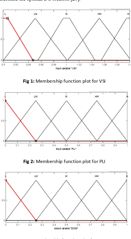
to be de-fuzzified using the centroid method in order to determine the optimal DG location [20].

Fig 1: Membership function plot for VSI

Fig 2: Membership function plot for PLI

Fig 3: Membership function plot for DGSI

4. STEPS FOLLOWED IN ALGORITHM

There are many computational steps involved in finding the optimal DG size and location to minimize losses in a radial distribution system are:

1. Run the load flow program. Select the bus where the maximum loss and low voltage is using fuzzy logic tool box. Corresponding DG size is calculated using Eq’s, respectively.

2. Repeat this for all the buses except the source bus. Identify the bus using the fuzzy logic that provides highest loss saving.

3. Compensate the bus with the highest loss with the corresponding DG unit found from Eq. (7).

4. Repeat the steps 1) and 2) to get the next DG size and hence sequence of buses to be compensated.

5. Once the sequence of buses is known determine the optimum DG unit sizes and the corresponding loss saving.

Since the system load is time variant and load duration curve of the system can be approximated .It is assumed that load level is constant. The above algorithm provides the optimal DG sizes and locations for a given load level.

5. RESULTS

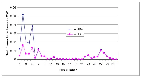
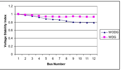
The proposed method is tested on three different test systems with different sizes, to show that it can be implemented in distribution systems of various configurations and sizes. The parameters of the first test system are given in Appendix. The second test system is 33-bus system [21], the total real power and reactive power loads on this system are 3.72 MW and 2.3 Mvar. The initial real and reactive power losses in the system are 0.211 MW and 0.143 Mvar. The third system is a 69-bus system [22], the total real power and reactive power loads on this system are 3.80 MW and 2.69 Mvar. The initial real and reactive power losses in the system are 0.225 MW and 0.102 Mvar. Based on the method described previously, the optimal sizes of DG are calculated at all buses for the three test systems. Fig. 4, Fig. 5 and Fig. 6 show the optimal sizes of Dg unit at all buses for 12, 33 and 69 bus distribution test systems, respectively. With the help of FIS editor optimal location of Dg unit is found where real power loss is more and voltage is low. The optimal locations of DG unit are bus9, bus6 and bus 61 for 12, 33 and 69 bus distribution test systems where total power losses attain the minimum value.

Fig 4: Optimal DG unit sizes for 12-bus radial distribution system

The real and reactive power losses for the corresponding optimal DG unit sizes are shown in Fig. 7, Fig. 8, Fig. 9, Fig. 10, Fig. 11

[image:4.612.59.287.91.506.2] [image:4.612.59.289.105.212.2] [image:4.612.329.547.434.562.2]

(5)

0 0.0005 0.001 0.0015 0.002 0.0025 0.003 0.0035 0.004 0.0045

1 2 3 4 5 6 7 8 9 10 11

Branch Number R e a l P ow e r Li ne Lo s s i n M W WODG WDG 0 0.0002 0.0004 0.0006 0.0008 0.001 0.0012 0.0014 0.0016 0.0018 0.002

1 2 3 4 5 6 7 8 9 10 11

Branch Number R e a c ti v e P ow e r Li ne Lo s s i n M v a r WODG WDG 0 0.5 1 1.5 2 2.5 3 3.5 4 4.5

1 3 5 7 9 11 13 15 17 19 21 23 25 27 29 31 33

Bus Number O pt im a l s iz e of D G i n M W

Fig 5: Optimal DG unit sizes for 33-bus radial distribution system 0 0.5 1 1.5 2 2.5 3 3.5 4 4.5

1 4 7 10 13 16 19 22 25 28 31 34 37 40 43 46 49 52 55 58 61 64 67

Bus Number S iz e of D G i n M W

[image:5.612.62.276.56.529.2]

Fig 6: Optimal DG unit sizes for 69-bus radial distribution system

Fig 7: Real power line losses of 12-bus radial distribution system with and without DG

Fig 8: Reactive power line losses of 12-bus radial distribution system with and without DG

0 0.01 0.02 0.03 0.04 0.05 0.06

1 3 5 7 9 11 13 15 17 19 21 23 25 27 29 31

[image:5.612.66.276.70.195.2]

Bus Number R e a l P ow e r Li ne Lo s s i n M W WODG WDG

0 0.005 0.01 0.015 0.02 0.025 0.03 0.035

1 3 5 7 9 11 13 15 17 19 21 23 25 27 29 31

[image:5.612.327.554.71.200.2]

Bus Number R e a c ti v e P ow e r Li ne Lo s s i n M v a r WODG WDG

Fig 10: Reactive power line losses of 33-bus radial distribution system with and without DG

0 0.01 0.02 0.03 0.04 0.05 0.06

[image:5.612.65.277.232.359.2]

1 4 7 10 13 16 19 22 25 28 31 34 37 40 43 46 49 52 55 58 61 64 67 Bus Number R e a l P ow e r Li ne Lo s s i n M W WODG WDG

0 0.002 0.004 0.006 0.008 0.01 0.012 0.014 0.016 0.018

[image:5.612.329.554.242.350.2]

1 4 7 10 13 16 19 22 25 28 31 34 37 40 43 46 49 52 55 58 61 64 67 Bus Number R e a c ti v e P ow e r Li ne Lo s s i n M v a r WODG WDG

[image:5.612.61.279.383.521.2] [image:5.612.333.550.400.507.2] [image:5.612.334.549.553.658.2] [image:5.612.56.281.557.687.2]

(6)

0 0.2 0.4 0.6 0.8 1 1.2

1 2 3 4 5 6 7 8 9 10 11 12

Bus Number

V

ol

ta

ge

S

ta

bi

li

ty

I

nd

e

x

[image:6.612.335.548.70.166.2]

WODG WDG

Fig 13: Voltage stability index of 12-bus radial distribution system with and without DG

0 0.2 0.4 0.6 0.8 1 1.2

1 3 5 7 9 11 13 15 17 19 21 23 25 27 29 31 33

Bus Number

V

ol

ta

ge

S

ta

bi

li

ty

I

nd

e

x

[image:6.612.62.274.72.194.2]

WODG WDG

0 0.2 0.4 0.6 0.8 1 1.2

1 4 7 10 13 16 19 22 25 28 31 34 37 40 43 46 49 52 55 58 61 64 67 Bus Number

V

ol

ta

ge

S

ta

bi

li

ty

I

nd

e

x

[image:6.612.326.553.212.654.2]

WODG WDG

[image:6.612.66.278.230.355.2]

Table 1 Results of critical bus analysis and comparison of active branch currents with and without DG for test systems

Ty pe

Bus no. corres

pondi ng to lowest voltag

e

Voltage in p.u. / VSI

Active branch current in branch1 in (A)

W.O. D.G

W.D. G

W.O.

D.G W.D.G

12-bus 12

0.9433 /0.792 0

0.982 3/0.93 11

41.42 15.76

33-bus 18

0.9037 /0.667 2

0.942 3/0.78 86

310.11 157.25

69-bus 61

0.9091 /0.683 3

0.981 7/0.92 88

318.09 159.18

Table-2 Results of proposed method for test systems

System Type 12-bus 33-bus 69-bus

Optimal location of DG

9-bus 6-bus 61-bus

Optimal DG

size in MW 0.22 2.59 1.87

Total real power loss in MW (WODG)

0.02069 0.2110 0.2250

Total reactive power loss in MVar (WODG)

0.00806 0.1430 0.1021

Total real power loss in MW (WDG)

0.01077 0.1110 0.0832

Total reactive power loss in MVar (WDG)

0.00415 0.0816 0.0405

Real power loss reduction in %

52.2 52.6 57.1

Reactive power loss reduction in

% 38.5 36.9 39.4

6. CONCLUSIONS

[image:6.612.64.279.402.507.2]

(7)

power and achieve significant improvement in voltage stability. Installation of DG unit at one location at a time is proved to be a valid assumption in the present study. However, this paper does not consider the other benefits of DG as well as economics of it.

7. REFERENCES

[1] Chowdhury S, Chowdhury SP, Crossley P.2009. Micro grids and Active Distribution Networks. 1st ed. London. IET Renewable Energy Series.

[2] Willis H. L, 2000. Analytical methods and rules of thumb for modeling DG distribution interaction. IEEE Proc. PES summer meeting, vol.3, pp. 1643-1644.

[3] Wang C, and Nehrir MH. 2004. Analytical approach for optimal placement of distributed generation sources in power systems. IEEE Trans. PWRS, 19(4), pp. 2068-2076. [4] Griffin T, Tomosovic K, Secrest D, and Law A. 2000

Placement of Dispersed Generation systems for reduced losses. In proceedings of 33rd Annual Hawaii International conference on systems sciences, Maui, Hawaii , pp. 1-9.

[5] Mardanesh M, and Gharehpattan GB. 2004. Siting and sizing of DG units using GA and OPF based technique. IEEE Region 10 Conference, 3: 331-34.

[6] Tripathy SC, Prasad GD, Malik OP, and Hope GS. 1982. Load flow solutions for Ill-conditioned power systems by a Newton-like method, IEEE Trans Power Ap Syst PAS-101 pp.3648-3657, D.O.I: 10.1049/ip-c: 19800043.

[7] Tinney WG and Hart CE. 1967. Power flow solutions by Newton’s method. IEEE Trans Power Ap Syst PAS-86; 1449-1457.

[8] Zhang F and Cheng CS. 1997.A modified Newton method for radial distribution system power flow analysis. IEEE Trans Power Syst 12 ; 389-397.

[9] Teng JH. 2002. A modified Gauss-Seidel algorithm of three-phase power flow analysis in distribution networks. Electric Power and Energy Systems 24; 97-102.

[10]Shirmohammadi D, Hong HW, Semlyen A and Luo GX. 1988. A compensation-based power flow method for weakly meshed distribution and transmission networks. IEEE Trans Power Syst 3, 753-762.

[11]Thukaram D, Banda HMW and Jerome J. 1999. A Robust three-phase power flow algorithm for radial distribution systems. Electric Power System Research 50, 227-236. [12]Ranjan R, Venkatesh B, Chaturvedi A and Das D. 2004.

Power flow solution of three-phase unbalanced radial distribution network. Electric Power Component Systems 32; 421-433.

[13]Teng JH. 2003. A direct approach for distribution system load flow solutions. IEEE Trans Power Deliver 18; 882-887.

[14]Kersting WH. 2002. Distribution system modeling and analysis, CRC Press, Boca Raton, FL.

[15]Cespedes R G. 1990. New method for the analysis of distribution networks. IEEE Trans Power Deliver 5; 391-396.

[16]Haque MH. 1996. Load flow solution of distribution systems with voltage dependent load models. Electric Power System Research 36; 151-156.

[17]Eminoglu U and Hocaoglu MH. 2005. A new power flow method for radial distribution systems including voltage dependent load models. Electric Power System Research; 106-114.

[18]Luo GX and Semlyen A. 1990. An Efficient load flow for large weakly meshed networks. IEEE Trans Power Syst, 1309_1316.

[19]Rajicic D, Ackovski R and Taleski R. 1994. Voltage correction power flow. IEEE Trans Power Delivery 9; 1056-1062.

[20]Fuzzy Logic Toolbox – MATLAB User’s Guide, Math works Inc.

[21]Kashem MA, Ganapathy V, Jasmon GB and Buhari M, 2000. A novel method for loss minimization in distribution networks. Proc. Int. Con. Electr. Util. Deregulation Restruct. Power Technol, April, 251-256.