R E S E A R C H
Open Access
Primal-dual interior point QP-free
algorithm for nonlinear constrained
optimization
Jinbao Jian
1, Hanjun Zeng
2, Guodong Ma
1*and Zhibin Zhu
3*Correspondence: [email protected] 1School of Mathematics and Statistics, Guangxi Colleges and Universities Key Laboratory of Complex System Optimization and Big Data Processing, Yulin Normal University, Yulin, China Full list of author information is available at the end of the article
Abstract
In this paper, a class of nonlinear constrained optimization problems with both inequality and equality constraints is discussed. Based on a simple and effective penalty parameter and the idea of primal-dual interior point methods, a QP-free algorithm for solving the discussed problems is presented. At each iteration, the algorithm needs to solve two or three reduced systems of linear equations with a common coefficient matrix, where a slightly new working set technique for judging the active set is used to construct the coefficient matrix, and the positive definiteness restriction on the Lagrangian Hessian estimate is relaxed. Under reasonable
conditions, the proposed algorithm is globally and superlinearly convergent. During the numerical experiments, by modifying the technique in Section 5 of (SIAM J. Optim. 14(1): 173-199, 2003), we introduce a slightly new computation measure for the Lagrangian Hessian estimate based on second order derivative information, which can satisfy the associated assumptions. Then, the proposed algorithm is tested and compared on 59 typical test problems, which shows that the proposed algorithm is promising.
MSC: 90C30; 49M37; 65K05
Keywords: inequality and equality constraints; optimization; primal-dual interior method; working set; global and superlinear convergence
1 Introduction
In this paper, we consider nonlinear constrained optimization problems with inequality and equality constraints
(P) minf(x), s.t. gi(x) = , i∈I; gj(x)≤, j∈Iı, ()
whereI={, , . . . ,m
},Iı={m+ ,m+ , . . . ,m+mı}, the functionsf andgj:Rn→R. It is known that the nonlinear equality constraints are difficult to be dealt with in design-ing algorithms for (P), especially, in designdesign-ing themethods of feasible directions(MFD). In , Mayne and Polak [] proposed a simple scheme to convert (P) to a sequence of inequality smoothing constrained optimization
(Pρ) minfρ(x) :=f(x) –ρ
j∈I
gj(x), s.t. gj(x)≤, j∈I∪Iı, ()
whereρ> is a penalty parameter. Under suitableconstraint qualifications(CQ), e.g., lin-ear independence, it has been shown that (Pρ) is equivalent to (P) whenρis large enough.
So, based on (Pρ), one can study and present effective algorithms for the original problem
(P), e.g., Refs. [, –].
In addition, with the help of inequality constrained non-smoothing optimization
min f(x) +
j∈I
cjgj(x), s.t. gj(x)≤, j∈I∪Iı,
one can also design an algorithm for solving the original problem (P), e.g., [], wherecj> is the penalty parameter that needs to be updated.
It is known that thesequential quadratic programming(SQP) method is one of the ef-ficient methods for constrained optimization due to its fast convergence, and it has been widely studied by many authors, see Refs. [–]. However, thequadratic program(QP) subproblems solved in the SQP methods may be inconsistent, and the computational cost for the QPs is high. Therefore, motivated by the KKT condition of the QPs and/or the quasi-Newton method, QP-free methods are put forward, in which the QPs are replaced by suitablesystems of linear equations(SLEs), see Refs. [–].
Now we review briefly the study on theprimal-dual interior point(PDIP) QP-free al-gorithms associated with our work. First, for problem (P) with no equality constraints, i.e.,I=∅, in , Panier et al. [] presented a QP-free algorithm denoted by PTH, at
iterate k, two SLEs are solved to yield a master search direction. Then aleast squares problem(LSP) needs to be solved to avoid the so-called Maratos effect []. However, the SLEs solved in [] may become ill-conditioned, and the PTH algorithm may be insta-ble. Furthermore, the initial point must lie on the strict interior of the feasible set, and an additional assumption that ‘the number of stationary points is finite’ is used to ensure the global convergence. Later, under the assumption that the multiplier approximation sequence remains bounded, the PTH algorithm was improved by Gao et al. [] by solv-ing an extra SLE. The PTH algorithm was also improved by Qi and Qi [], Zhu [] and Cai [].
To improve the PTH algorithm [], by using the idea of PDIP and choosing different barrier parameters for each constraint, Bakthiari and Tits [] proposed a new PDIP QP-free algorithm. The algorithm can start from a feasible point at the boundary of the feasible set, and it possesses global convergence without both the additional assumption of isolat-edness of the stationary points and the positive definite restriction on matrixHk. Almost at the same time, Tits et al. [] extended and improved the PTH algorithm to problem (P) with both inequality and equality constraints. The algorithm [] possesses two remarkable characters. One is that a new and simple rule to update the penalty parameterρin (Pρ) is
derived, the other is that, same as in [], the uniformly positive definite restriction on the Lagrangian Hessian estimate is relaxed.
relaxed; at each iteration, only two or three SLEs with the same coefficient matrix needed to be solved.
However, there are still some problems worthy of research on the PDIP-type algorithms [, , ]. First, the coefficient matrix of the Karush-Kuhn-Tucker (KKT) system of the LSP is not the same as the two previous SLEs, and this further increases the computa-tional cost. Second, the coefficient matrices of the SLEs include all the constraints and their gradients, and this leads to a large increase in the scale of the SLEs. Third, the global convergence of the two algorithms [, ] relies on an additional assumption that the sta-tionary points are finite or isolated.
On the other hand, to design more effective algorithms with small computational cost for solving constrained optimization, Facchinei et al. [] first introduced the active set identifying technique (also called working set technique). And then this technique has been popularized and applied in many works, e.g., [, , , , ]. Particularly, the algorithm [] needs to solve four SLEs at each iteration.
The goal of this paper is to improve and extend the algorithms [, ] to nonlinear constrained optimization (P) and, at the same time, to overcome the three problems men-tioned above. As a result, by means of problem (Pρ), we propose a PDIP-type algorithm for
problem (P). Compared with the previous PDIP-type algorithms, the proposed algorithm possesses the following features.
(a) A slightly new identifying technique for the active set different from [, ] is introduced. The multiplier yielded at the previous iteration is used to compute the working set, and no additional computational cost is needed, so the computational cost is expected to be reduced.
(b) At each iteration, to yield the search directions, only two or three SLEs with the same coefficient matrix need to be solved. Furthermore, the coefficient matrix has smaller scale than the ones in [, , ].
(c) For a strict interior pointxkof the feasible set of (P
ρ), the iteration atxkis well
defined without any other constraint qualification (CQ).
(d) Under suitable CQ and assumptions including a relaxed positive definite restriction on the Lagrangian Hessian estimateHk,but without the isolatedness of the
stationary points, the proposed algorithm is globally and superlinearly convergent. (e) A slightly new computation technique forHkbased on second order derivative
information is introduced, which is a modification of the one in [], Section ., and satisfies the relaxed positive definite restriction.
Throughout this paper, for simplicity, denote vector (xT,yT,zT, . . .)T by (x,y,z, . . .) for column vectorsx,yandz, and · denotes the Euclidean norm.
2 Construction of algorithm
To analyze our algorithm, the following notations are used:
I=I∪Iı, eˆ=, . . . , (mth), , . . . ,
(m+mı)th
T ,
X=x∈Rn:gi(x) = ,i∈I;gj(x)≤,j∈Iı, eJ= (, . . . , )T∈R|J|,
˜
X=x∈Rn:gj(x)≤,j∈I, X˜=
x∈Rn:gj(x) < ,j∈I,
I(x) =j∈I:gj(x) = , Iı(x) =j∈Iı:gj(x) = , I(x) =I(x)∪Iı(x),
g(x) =
gj(x),j∈I, gı(x) =
gJ(x) =
gj(x),j∈J⊂I, ∇gJ(x) =
∇gj(x),j∈J,
gjk=gj
xk, gJk=gJ
xk, ∇gjk=∇gj
xk, ∇gjkT=∇gjkT.
First, the following basic hypothesis is necessary.
H The inner setX˜is nonempty, and the functionsf andgj(j∈I) are all continuously
differentiable.
Remark Note that if there exists a point belonging to the setX˜, namely,xˆ∈ ˜X, and the active constraint gradient vectors{∇gj(xˆ),j∈I(xˆ)}are linearly independent, then one can yield a pointx∈ ˜Xby simple computation, e.g., execute line search ongstarting withxˆ along directiondˆ= –Nˆ(NˆTNˆ)–e, whereNˆ =∇g
I(xˆ)(xˆ) ande= (, . . . , )T.
Before proposing our algorithm, we give a proposition to show the equivalences between (P) and (Pρ).
Proposition If(x,λ)is a KKT pair for problem(Pρ)and g(x) = ,then(x,λρ)with mul-tiplierλρ=λ–ρˆe is a KKT pair for the original problem(P).
Based on Proposition , it is known that if one can construct an effective algorithm for problem (Pρ) and adjust parameterρto force the iterate to asymptotically satisfyg(x) = ,
then the solution to (P) can be yielded.
Now, refer to [] and [], we introduce optimal identification functionsandδas follows:
(x,λ) = ⎛ ⎜ ⎝
∇xL(x,λ)
g(x)
min{–gı(x),λı}
⎞ ⎟
⎠, δ(x,λ) =(x,λ)r, ()
whereλ= (λ,λı), parameterr∈(, ), and the Lagrangian function
L(x,λ) =f(x) + j∈I
λjgj(x). ()
It is clear that (x∗,λ) is a KKT pair of (P) if and only ifδ(x∗,λ) = . Particularly, from [] or/and [], Definition ., Theorems ., . and ., one can see that{j∈I:gj(x) + δ(x,λ)≥}is an exact identification set for active constrain setI(x∗) if (x,λ) converges to a KKT pair (x∗,λ) of problem (P), and the Mangasarian-Fromovotz constraint qualification (MFCQ) and the second order sufficient conditions are satisfied at (x∗,λ).
In this paper, similarly to the techniques in [, ], for the current iteratexk∈ ˜X , we yield the corresponding multiplier vectorλk= (λk,λkı) in ()-() as follows:
λ=z, λk=λ¯k––ρk–eˆ, k> , ()
wherez> , and (λ¯k–,ρ
k–) is computed in the previous iteration (k– )th. Then, similarly to [], we structure our working set by
Ikı=j∈Iı:gj
The reason why one does not computeI
k asIkı is to forceg(xk)→, see the analysis
of Theorem in Section . The setIı
k equals the exact active setI
ı(x∗) when (xk,λk) is
sufficiently close to a KKT pair (x∗,λ) of (P) and the second order sufficient conditions as well as the MFCQ hold at (x∗,λ). This important property allows us to construct the direction finding subproblems only considering the constraints in the working setIk.
Taking into account that the iterates always execute within the feasible setX˜, let us con-sider the first order condition of optimality (KKT condition) for problem (Pρk) nearby the current iteratexk:
∇fρk(x) +
j∈Ik
λj∇gj(x) = , λjgj(x) = , j∈Ik,λIk≥.
Furthermore, if we ignore the non-negativity request ‘λIk≥’ and simultaneously intro-duce a suitable perturbation (( –ζk)∇fρk(x
k),μk)∈R(n+|Ik|) in the right-hand side of the
above system, then it can be reduced as a system of nonlinear equations with variables (x,λIk)
∇fρk(x) +
j∈Ikλj∇gj(x) λjgj(x),j∈Ik
=
( –ζk)∇fρk(x k)
μk
. ()
Applying the Newton method to system () starting with the current iterate (xk,λk Ik), it yields a SLE as follows:
∇ xxLρk(x
k,λk
Ik) ∇gIk(x k)
k∇gIk(xk)T diag(gIkk)
x–xk λIk
=
–ζk∇fρk(x k)
μk
, ()
where diagonal matrixk=diag(λkIk), and the Lagrangian Hessian
∇ xxLρk
xk,λkIk=∇fρk
xk+ j∈Ik
λkj∇gj
xk.
Subsequently, to make the coefficient matrix in SLE () possess nice property and low computational cost, we consider its optimization and modification as follows. First, re-place the Lagrangian Hessian by a suitable approximate symmetric matrixHk, and denote
x–xkby directiond. Second, replace the diagonal matrix
kby positive diagonal matrix
Zk=diag(zkIk), where vectorz k
Ik is an approximation ofλ k.
As a result, from system (), the coefficient matrix and the form of the SLEs that need to be solved in our algorithm are as follows:
Vk:=
Hk ∇gIk(x k)
Zk∇gIk(xk)T diag(gIkk)
, ()
SLEVk;ζk,μk: Vk
d
λIk
=
–ζk∇fρk(x k)
μk
. ()
Subsequently, it is necessary to analyze the singularities of the coefficient matrix Vk above, i.e., the solvability of SLE ().
Lemma For iterate xk∈ ˜Xand zkIk> ,if the matrix Hksatisfies
Hk
j∈Ik
zjk
gjk∇g
k j∇gk
T
j , ()
then the coefficient matrix Vkdefined by()is invertible,where matrix order AB means (A–B)is positive definite on Rn.
Proof One knows that it is sufficient to show that SLEVku= has a unique solution zero,
and this is elementary and omitted here.
Remark Obviously, the positive definiteness request () onHkis weaker than the pos-itive definiteness ofHkitself onRn. But it is stronger than the positive definiteness ofHk on the null space of the gradients of approximate active constraints, i.e., on k:={d∈Rn:
∇gIk(xk)Td= }. However, the latter cannot ensure the invertibility ofVk.
Based on the above analysis and preparation, now we can describe the steps of our al-gorithm solving (P) as follows.
Algorithm A
Parameters: α∈(,),σ,β,θ,r∈(, ),ξ∈(, ), ν> ,ϑ> ,M,p> ; suitable small positive parametersγ,γ andγ; sufficiently small lower boundε> and sufficiently large upper boundε> ; termination accuracy> .
Data: x∈ ˜X
,ρ> , vectorszwith weightszj∈[ε,ε],j∈I. Setk:= .
Step Compute working set. Computeλk by (),(xk,λk) andδ(xk,λk) by ()-(). If (xk,λk)≤or other suitable termination rule is satisfied, then (xk,λk) is an approximate KKT pair of problem (P) and stop; otherwise, generate the working setsIı
kandIkby ().
Step Yield matrix Hk. Yield matrixHksuch that it approximates to the Hessian of the Lagrangian associated with (Pρk) and satisfies request ().
Step Compute the main search directions.
(i) Compute (d¯k,λ¯kIk) by solvingSLE(Vk; , ), see (), then setλ¯k= (λ¯kIk, I\Ik) = (λ¯k,λ¯kı)
withλ¯k
ı = (λ¯kIkı, Iı\Ikı).
(ii) Check conditions: (a) ¯dk ≤γ
, (b)λ¯k≥–γeI, (c)λ¯k≯γeI. If all the three con-ditions above hold, then increase penalty parameterρbyρk+=ϑρk, setxk+=xk,zk+=
zk,H
k+=Hk,Ikı+=I
ı
k,Ik+=Ik,k:=k+ , and go back to Step (i). Otherwise, setρk+=ρk, proceed to Step (iii) as follows.
(iii) Yield the weights of vectorφkby
φkj =min, –max–λ¯jk, p–Mgjk, j∈Ik. ()
Then compute
ξk=∇fρk
xkTd¯k– j∈Ik
¯
λk jφjk
zk j
bk=d¯k
ν
+φk
j∈Ik
¯
λkj
+
j∈Ik
¯
λkj
zkj φ
k
j, ()
ϕk= ⎧ ⎨ ⎩
, ifbk≤;
min{(–θ)|ξk|
bk , }, ifbk> ,
()
and yield perturbation vectors via convex combinations
μk= ( –ϕk)φk+ϕk
–d¯kν–φkzkIk. ()
(iv) Compute (dk,λkIk) by solving SLE(Vk; ,μk), see (), then set λk = (λkIk, I\Ik) = (λk,λkı) withλkı = (λkIı
k, I ı\Iı
k).
Step Trial of unit step.If
fρk
xk+dk≤fρk
xk+α∇fρk
xkTdk, gj
xk+dk< , ∀j∈I,
then let the step sizetk= , the high order correction directiond˜k= , and enter Step . Otherwise, proceed to Step .
Step Generate high order correction direction.Compute (d˜k,λ˜k
Ik) by solvingSLE(Vk; ,μ˜k), where
˜
μk= –ωkeIk–ZkgIk
xk+dk, ()
ωk=max
dkξ;dkmax – z k j
λkj
σ,j∈Ik,λkj =
. ()
If˜dk>dk, resetd˜k= .
Step Perform arc search.Compute the step sizetk, the maximum numbertof sequence
{,β,β, . . .}satisfying
fρk
xk+tdk+td˜k≤fρk
xk+αt∇fρk
xkTdk, ()
gj
xk+tdk+td˜k< , j∈I. ()
Step Update.Yield a new iterate byxk+=xk+t
kdk+tkd˜kand compute
zk+ j =min
maxdk+ε,λk j
,ε, j∈I. ()
Setk:=k+ , go back to Step .
Subsequently, we analyze and describe some properties of Algorithm A by the following lemma and several remarks. For convenience of writing, denote matrix
Qk:=Hk–
j∈Ik
zk j
gk j
∇gk j∇gk
T
j . ()
Lemma For the directionsd¯kand dkyielded in Step(i), (iv),the following two relations
hold:
∇fρk
xkTd¯k= –d¯kTQkd¯k≤, ∀k≥, ()
∇fρk
xkTdk≤θ ξk≤, ∀k≥. ()
Furthermore,when the iterative process goes into Step(iii), (iv),one hasd¯k= andξk< ,
so dkis a feasible direction of descent of problem(P
ρk)at point xkand the arc search in Step can be finished by finite calculations.Therefore,AlgorithmAis well defined.
Proof First, from () andSLE(Vk; , ) (), we have
∇fρk
xkTd¯k= –d¯kT
Hkd¯k+
j∈Ik
∇gk jλ¯kj
= –d¯kT
Hk–
j∈Ik
zkj
gjk∇g
k j∇gk
T j
¯ dk
= –d¯kTQkd¯k≤.
So, conclusion () is at hand. Second, from ()-(), one gets
φjkλ¯kj ≥, ∀j∈Ik; ξk≤ ∇fρk
xkTd¯k≤. ()
On the other hand, taking into accountSLE(Vk; , ) andSLE(Vk; ,μk) as well as ()-(), it is not difficult to show that
∇fρk
xkTdk=∇f
ρk
xkTd¯k– j∈Ik
¯
λkjμkj
zkj =ξk+ϕkbk. ()
Again, in view of (), it follows thatϕkbk=bk≤ ifbk≤, hence, the relationsξk+ϕkbk≤ ξk≤θ ξkhold sinceξk≤. Ifbk> , thenξk+ϕkbk≤ξk+ (θ– )ξk=θ ξk. In all, one gets
ξk+ϕkbk≤θ ξk. This, together with () and (), shows that∇fρk(x
k)Tdk≤θ ξ k≤. Third, ifd¯k= , then, fromSLE(Vk; , ) (),g(xk) < and (), it follows thatλ¯k
Ik= . So, by the structure of Step , the iteratekdoes not go into Step (iii), (iv). Thus,d¯k= when the iterative process goes into Step (iii), (iv).
Finally,ξk< follows from (), () andd¯k= . The remaining claims in Lemma are
at hand byξk< andg(xk) < .
As an end of this section, to help the readers understand our algorithm, we further an-alyze the steps/structure of Algorithm A with three remarks below.
Remark (Analysis for Step )
(i) The role of solvingSLE(Vk; , )with no perturbation in Step (i) is to check whether the current iteratexkis an approximate KKT point of (P
ρk) and yield an
(ii) If conditions (a) and (b) in Step (ii) are satisfied, and the parametersγandγare
small enough, thenSLE(Vk; , )implies thatxkis an approximate KKT point of
(Pρk). However, if case (c) is also satisfied, one cannot estimateg(x
k). So, we
increase the penalty parameterρ. In practical computation, if conditions (a) and (b) are satisfied andg(xk)is small enough, we can terminate the algorithm.
(iii) From result (), one knows thatd¯kis a descent direction of the merit function
fρk(x)atx
kwhend¯k= . However, the primal feasibility and dual feasibility are
relaxed to a large extent inSLE(Vk; , ),d¯kcannot be used as an effective search
direction. So, generally, the first directiond¯kshould be corrected by another SLE.
For this goal, refer to [], we construct and solveSLE(Vk; ,μk)in Step (iii), (iv). Lemma and the global convergence analysis in the next section show that the algorithm with search directiondkis well defined and globally convergent.
Remark (Explanation for Steps and ) Usually, search directiondkcannot avoid the Maratos effect, i.e., unit step cannot be accepted by the associated line search for all suf-ficiently large iteratesk. So, to overcome the Maratos effect and obtain superlinear con-vergence, one needs to compute an additional high order correction direction. Here, we generate it by solvingSLE(Vk; ,μ˜k) in Step . Obviously, solvingSLE(Vk; ,μ˜k) should add computational cost more or less. On the other hand, numerical testing shows thatdk can still avoid the Maratos effect at some iterates. Therefore, to save computational cost as much as possible, the trial of unit step in Step is added.
Remark With the help of the working set technique, the three SLEs solved in
Algo-rithm A have a common coefficient matrixVk, which can save the cost of computation
and is different from those in Refs. [, ], etc. Furthermore, due to being interior point type and the constructing technique forVk, Algorithm A is well defined at each iterate without any other CQ except the strict innerX˜=∅, see Lemmas and . In many ex-isting QP-free type algorithms, see Refs. [, , –], the linearly independent constraint qualification (LICQ) is necessary to ensure the iterate itself is well defined. Of course, as we see in Assumption H, to obtain the global and superlinear convergence of Algorithm A, a suitable CQ on the boundary ofX˜ is still necessary.
3 Analysis of global convergence
In this section, we assume that the proposed algorithm (Algorithm A) generates an infinite iteration sequence{xk}of points. First, we show that the penalty parameterρ
kcan be fixed after finite iterates. And then, we prove that Algorithm A is globally convergent. For this goal, the following hypotheses are necessary.
H Suppose that the sequences both{xk}and{H
k}yielded by Algorithm A are bounded,
and assume that there exists a positive constantasuch that
dTHkd≥ad–
j∈Ik
zk j
|gk j|
∇gkT j d
, ()
i.e.,dTQ
kd≥ad,∀k,∀d∈Rn.
(i) the gradient vectors{∇gj(x),j∈I(x)}are linearly independent; and (ii) ifx∈/X, i.e.,g(x)= , then there exist no scalarsλj≥,j∈I(x)such that
j∈I∇gj(x) =
j∈I(x)λj∇gj(x).
Remark (Analysis for H) The uniform ‘positive-definiteness’ request () on{Hk}is weaker than the usual uniform positive-definiteness of{Hk}itself onRn, namely,dTHkd≥
ad,∀k,∀d∈Rn. However, it is stronger than the uniform positive-definiteness ofH kon the null space k. It is encouraging that, based on the Lagrangian Hessian, we can design an alternative computational technique for Hk such that{Hk} is bounded and satisfies request (), which implies () whenever{xk}is bounded, see formulas (), () and () as well as Theorem in Section .
Remark (Analysis for H)
(i) Hypothesis H was introduced by Tits et al. in [], Assumption . In our work, it plays two roles in the convergence analysis of Algorithm A. One is to ensure the correction for the penalty parameterρcan be finished in a finite number of iterations, the other is to assure that the sequence{Vk}of coefficient matrices is
uniform invertible, see Lemmas and . Furthermore, H is considerably milder than the linear independence of the gradients{∇gi(x),i∈I;∇gj(x),j∈Iı(x)}, a
detailed analysis for this assumption can be seen in [, ].
(ii) First, H automatically holds at each interior pointx∈ ˜X. Second, H can be
reduced to each accumulation pointx∗of the iterate sequence{xk}, which satisfies
x∗∈ ˜/X. However, the latter is difficult to be verified.
Lemma Suppose that H, HandHhold.Then the penalty parameterρk in
Algo-rithmAis increased at most finite times.
The proof of Lemma is similar to the one of [], Lemma ., and omitted here. In what follows,ρ¯denotes the final value ofρk, i.e.,ρk≡ ¯ρwhenkis sufficiently large.
Lemma Suppose thatH, HandHhold.Then
(i) the sequence{Vk}of coefficient matrices is unified invertible,i.e.,there exists a
positive constantM¯ such thatV–
k ≤ ¯M,∀k≥,and
(ii) both sequences{(d¯k,λ¯k)}and{(dk,λk)}are bounded.
Proof (i) By contradiction, suppose that there exists an infinite subset K such that
V–
k
K
→ ∞. In view of the boundedness of{xk}and{Hk}, Step and the finite choice ofIkı, without loss of generality, fork∈K, assume that
Ikı≡I, xk→x∗, Hk→H∗, zk→z∗≥εeI> .
DenoteˆI=I∪IandZ
∗=diag(z∗ˆI), then
Vk K
→V∗:=
H∗ ∇gIˆ(x∗) Z∗∇gˆI(x∗)T diag(gIˆ(x∗))
. ()
Consequently, under H-H, refer to the proof of [], Lemma .(i), one can show that
V∗is nonsingular. SoVk– K
→ V–
∗ <∞, which contradictsVk– K
(ii) First, the boundedness of{(d¯k,λ¯k)}follows fromSLE(Vk; , ) and conclusion (i) as well asρk≡ ¯ρ. Second, the boundedness of{μk}follows from formulas ()-() and the boundedness of{(d¯k,λ¯k)}as well as the positive boundary below of{zk}. Therefore, the
boundedness of{(dk,λk)}is also at hand bySLE(Vk; ,μk).
Lemma Suppose thatH, HandHhold.Let x∗be an accumulation point of the se-quence{xk}generated by AlgorithmA,and suppose that{xk}
K→x∗for some infinite index
set K.If{ξk}K→,then x∗ is a KKT point of problem(Pρ¯),and both{¯λk}K and{λk}K
converge to the unique multiplier vectorλ∗associated with x∗.
Proof Let (λ¯∗;λ) be any given limit point ofˆ {(λ¯k;λk)}K. We first show that (x∗,λ¯∗) is a KKT pair of (Pρ¯). In view of H, Lemma and the finite choice ofIkı, we know that there is an
infinite indexK⊆Ksuch that
Ikı≡I, λ¯k;λk→λ¯∗;λˆ,
Hk→H∗, d¯k→ ¯d∗, zk→z∗≥εeI, k∈K.
()
Therefore, from (), () and H, one can easily getd¯∗= by{ξk}K→. Further, taking the limit inSLE(Vk; , ) fork∈K, we have, hereˆI=I∪I,
∇fρ¯
x∗+
j∈ˆI
¯
λ∗j∇gj
x∗= ; λ¯∗jgj
x∗= , ∀j∈ ˆI. ()
Next, divert our attention to showing thatλ¯∗≥. It is obvious thatλ¯∗j = follows from
¯
λ∗jgj(x∗) = forj∈ ˆI\I(x∗). Moreover, from the definition ofξk, i.e., (), and (ξk,d¯k)→K
(, ), we can deduce thatj∈ˆIλ¯ k jφjk
zkj →,k∈K
. Further, in view of (), we know that each
term λ¯ k jφjk
zjk ≤, which together with () implies thatλ¯ k jφjk
K
→. This, plus (), shows that
¯
λ∗jmin{, –(max{–λ¯∗j, })p–Mgj(x∗)}= forj∈ ˆI, and this includesλ¯∗
j ≥ forj∈ ˆI∩I(x∗). Therefore,λ¯∗ˆ
I ≥. Obviously,λ¯
∗
I\ˆI= . Soλ¯
∗≥ is at hand.
Hence, taking into accountx∗∈ ˜X, we can conclude from () that (x∗,λ¯∗) is a KKT pair andx∗ is a KKT point for (Pρ¯). Furthermore, the analysis above further shows that the
sequence{¯λk}K possesses a unique limit point, i.e., the unique KKT multiplier vectorλ∗. Solimk∈Kλ¯k=λ∗.
Finally, taking into account (d¯k,λ¯k)→K (,λ∗)≥, from () and (), we have (φk,
μk)→K . Therefore,SLE(Vk; ,μk) minusSLE(Vk; , ) gives
Vk
dk–d¯k
λkˆ I –λ¯
k
ˆ
I
=
μk
K
−→
. ()
This, along with Lemma (i), shows thatλˆ=limk∈Kλk=limk∈Kλ¯k=λ∗.
Theorem Suppose thatH, HandHhold.Then each accumulation point x∗ of the sequence {xk} generated by AlgorithmA is a KKT point of the original problem(P),i.e.
Proof First, there exists an infinite index setKsuch thatxk→x∗,k∈K, and relation () holds. By contradiction, suppose thatx∗is not a KKT point of (P). Then, from Lemma , without loss of generality, one can suppose thatλk=λ¯k––ρ¯eˆ→ ¯λ,k∈K. Therefore, it follows that (x∗,λ¯) is not a KKT pair of (P), which further implies thatδ(x∗,λ¯) > and
Iı(x∗)⊆Iı
k,k∈Klarge enough. There are two cases as follows to be considered.
Case I: Assume thatx∗is a KKT point of (Pρ¯). Then there exists a multiplierλ¯≥ such
that the KKT condition of (Pρ¯) is satisfied at (x∗,λ¯). In view ofIı(x∗)⊆Ikı ≡Iholds for k∈Klarge enough, it is easy to know, from the KKT condition of (Pρ¯), that (,λ¯I∗) is a solution to SLE in (u,v)
V∗
u v
=
–∇fρ¯(x∗)
, ()
where matrixV∗is defined by (). On the other hand, passing to the limit inSLE(Vk; , )
fork∈Kandk→ ∞, one knows that (d¯∗,λ¯∗I∗) also solves system () above. Taking into account the nonsingularity of matrixV∗(by Lemma (i)), one knows that the solution of () is unique. Sod¯∗= andλ¯∗I∗=λ¯I∗≥, which impliesλ¯∗=λ¯≥ . Thus, conditions (a) and (b) in Step (ii) are always satisfied fork∈Klarge enough. Therefore, in view of ρk≡ ¯ρ<∞forklarge enough, Step (ii) impliesλ¯kI>γeIfork∈Klarge enough, which further implies thatλ¯∗
I≥γeI> . Hence, it follows from the complementary slackness at KKT pair (x∗,λ¯), =λ¯jgj(x∗) =λ¯∗jgj(x∗) = (j∈I). Sog
(x∗) = , which together with
Proposition implies thatx∗is also a KKT point of (P), which contradicts the assumption thatx∗is not a KKT point of (P).
Case II: Suppose thatx∗is not a KKT point of (Pρ¯). And, by Lemma andξk≤, one can deduce thatξk→ ¯ξ< ,k∈K. Further, this along with () and () as well as H, shows thatlimk∈K(¯dkν+φk) > . So there exist a subsetK⊆Kand a positive constant such that
ξk≤ ¯ξ/ < , d¯k
ν
+φk≥> , k∈K.
The remaining proof is divided into two steps.
Step A:Show that there exists a constantt¯> such that the step-lengthtk≥ ¯tholds for allk∈K.
(A) Analyze inequality (). First, for j∈/ I(x∗),gj(x∗) < , from the boundedness of
{(dk,d˜k)}
K and the continuity ofgj, one gets thatgj(xk+tdk+td˜k) < holds fork∈K large enough andt> sufficiently small. Second, consider indexj∈I(x∗), i.e.,gj(x∗) = . In view ofIı(x∗)⊆Iı
k, which impliesj∈Ik, from Taylor expansion, formulas (), () and SLE(Vk; ,μk) as well as˜dk ≤ ¯dk, fort> small enough, we obtain that
gj
xk+tdk+td˜k=gjk+t∇gjkTdk+o(t) =gjk+tμ
k j–λkjgjk
zjk +o(t)
=
–tλ
k j
zk j
gjk+t –ϕk zk
j
φjk–tϕkd¯k
ν
+φk+o(t)
≤–tϕkd¯k
ν
+φk+o(t),
On the other hand, taking into accountξk≤ ¯ξ/ < and the boundedness ofbk() (by Lemma ) as well as (), we know that there exists a constantϕ> such thatϕk≥ϕ> ,k∈K. Sogj(xk+tdk+td˜k)≤–ϕt+o(t) < holds fork∈Klarge enough andt> sufficiently small. Therefore, inequality () holds fort> sufficiently small andk∈K
large enough.
(A) Analyze inequality (). From Taylor expansion and (), one gets
fρ¯
xk+tdk+td˜k–fρ¯
xk–αt∇fρ¯
xkTdk= ( –α)t∇fρ¯
xkTdk+o(t)
≤( –α)tθ ξk+o(t)
≤( –α)tθξ¯/ +o(t)
≤.
Hence, inequality () holds fork∈Klarge enough andt> sufficiently small. Up to now, one can conclude that there exists a constant¯t> such thattk≥ ¯tfor eachk∈K.
Step B:Usetk≥ ¯t> (k∈K) to bring a contradiction. Because oflimk∈Kfρ¯(xk) =fρ¯(x∗)
and the monotone property of{fρ¯(xk)}, one knows thatlimk→∞fρ¯(xk) =fρ¯(x∗). Further, in
view of () and (), it follows that fork∈Klarge enough
fρ¯
xk+–fρ¯
xk≤αtk∇fρ¯
xkTdk≤αtkθ ξk≤αθξ¯¯t/.
Passing to the limit fork∈Kandk→ ∞in the inequality above, we can bring a con-tradiction. Summarizing the discussions above, the whole proof of Theorem is
com-pleted.
4 Analysis of strong and superlinear convergence
In this part, under some additional mild assumptions, we first show that the proposed algorithm is strongly convergent, that is, the whole sequence{xk}is convergent. Then the unit step can be accepted and the Maratos effect can be avoided for allklarge enough. At last, we prove that Algorithm A achieves superlinear convergence.
H (i) The functionsf(x)andg(x)are all twice continuously differentiable overX˜; and (ii) there exists an accumulation pointx∗of the sequence{xk}of iterative points
with (unique) KKT multiplierλassociated with (P) such that the second order sufficiency conditions (SOSC) and the strict complementarity hold, i.e., the KKT pair(x∗,λ)of (P) satisfiesλIı(x∗)> and
dT∇xxLx∗,λd> , ∀d∈d∈Rn:d= ,∇gI(x∗)
x∗Td= .
Remark Denote the Lagrangian function of problem (Pρ¯) byLρ¯(x,λ) =fρ¯(x) +
j∈Iλj×
gj(x). Then, with relationλρ¯ =λ–ρ¯eˆ, we haveL(x,λρ¯) =Lρ¯(x,λ). Therefore, taking into
account Lemma (iv), it is readily checked that the SOSC with the strict complementarity for (Pρ¯) is identical with that for (P).
Lemma Suppose thatX˜ =∅and assumptionsH, HandHare satisfied(by Remark,
˜
X=∅plusH(i)impliesX˜= ∅).Then,for any subset K such that{xk}K converges to the
(i) Iı(x∗)⊆Iı
kfork∈Ksufficiently large;
(ii) x∗is a KKT point of problem(Pρ¯);
(iii) {(d¯k,λ¯k)}
K→(,λ∗)and{(dk,λk)}K→(,λ∗),whereλ∗together withx∗is a KKT
pair of problem(Pρ¯);and
(iv) the KKT multiplierλof(P)andλ∗of(Pρ¯)associated with the KKT pointx∗satisfy
λ=λ∗–ρ¯eˆ,λ∗I(x∗)> .
Proof (i) From Lemma (ii), there exists an infinite subsetK⊆Ksuch that
xk→x∗, λk=λ¯k––ρ¯eˆ→ ¯λ, k∈K.
If (x∗,λ¯) is a KKT pair of (P), thenλ¯=λ¯∗. Further, under H, by [, ], one knows that
Iı
k≡I
ı(x∗) fork∈Klarge enough. Otherwise, we have <δ(x∗,λ¯)←K δ(xk,λk). So, from
(),Iı(x∗)⊆Iı
kalso holds fork∈Klarge enough.
(ii) By contradiction, suppose thatx∗is not a KKT point of (Pρ¯). Then, taking into
ac-count conclusionIı(x∗)⊆Iı
k(k∈Klarge enough), by Case II of the proof of Theorem , we can bring a contradiction.
(iii) To show{(d¯k,λ¯k)}K→(,λ∗), it is sufficient to show that (,λ∗) is a unique accumu-lation point of{(d¯k,λ¯k)}
K. Let (d¯,λ) be any given accumulation point of¯ {(d¯k,λ¯k)}K. Since the sequences{(d¯k,λ¯k)}and{zk}are all bounded, in view of H, H andIı
k⊆I
ı, there exists
an infinite subsetK⊆Ksuch that
Ikı≡I, Hk→H∗, d¯k,λ¯k→(d¯,λ),¯ zk→z∗, k∈K. ()
Now, passing to the limit fork∈Kandk→ ∞inSLE(Vk; , ), we deduce that (d¯,λ¯ˆI) (Iˆ:=I∪I) solves SLE (). Further, it follows from Lemma (i) that the coefficient matrix
of SLE () is nonsingular. Thus the solution of () is unique. On the other hand, in view ofIı(x∗)⊆I,I(x∗) =Iand (x∗,λ∗) being a KKT pair of (P
¯
ρ), we know that (,λ∗Iˆ) is also a
solution to system (). Therefore (d¯,λ¯ˆI) = (,λI∗ˆ), this further implies that (d¯,λ) = (,¯ λ ∗)
and (,λ∗) is a unique limit point of{(d¯k,λ¯k)} K. Finally, conclusion{(dk,λk)}
K→(,λ∗) follows from{(d¯k,λ¯k)}K→(,λ∗) and (). (iv) By Proposition andg(x∗) = , we haveλ=λ∗–ρ¯ˆe, andλ∗Iı(x∗)=λIı(x∗)> by H(ii). Further, in view ofd¯k→,λ¯k→λ∗≥,k∈K, one knows that conditions (a) and (b) in Step (ii) hold forklarge enough. Therefore, taking into accountρk≡ ¯ρforklarge enough, it follows thatλ¯k>γe
Iby Step (ii), soλ∗≥γeI> . Thereforeλ∗I(x∗)> holds.
Remark In view ofI(x∗) =I, from H, H and Lemma (ii), (iv), the following
con-clusion holds: The LICQ, SOSC and strict complementarity of problem (P) and problem (Pρ¯) are satisfied at their KKT pair (x∗,λ) and (x∗,λ∗), respectively.
In view of Remark , similarly to the proof of [], Theorem ., Lemma ., we have the following result.
Theorem Suppose thatX˜ =∅and assumptionsH, HandHare satisfied.Then
(i) xk→x∗,i.e.,AlgorithmAis strongly convergent;
(ii) (d¯k,λ¯k)→(,λ∗), (dk,λk)→(,λ∗),zk→min{max{εeI,λ∗},εeI},and
(iii) φk= ,μk= –ϕ
Lemma Suppose that the hypotheses in Lemmahold,and assume that the boundary parametersεandεsatisfy
ε≤minλ∗j,j∈I∗, ε≥maxλ∗j,j∈I∗
. ()
Then
zIk∗→λ∗I∗, ωk=odk, ()
and the solution(d˜k,λ˜k
I∗)ofSLE(Vk; ,μ˜k)satisfies
d˜k,λ˜Ik∗=O(ωˆk) =odk, ωˆkdk=o(ωk), ()
where
ˆ
ωk=maxzkj/λkj – ·dk,j∈I∗;dk
. ()
Furthermore, the correction direction d˜k in Stepis always yielded by the solution of SLE(Vk; ,μ˜k).
Proof First, from the given conditions and Theorem (iv), relationzk
I∗→λ∗I∗ is at hand. Further, this, together with Theorem (ii), shows thatzkj/λkj → forj∈I∗. So, it follows
thatωk=o(dk) from ().
Second, we prove relation (). From Theorem (ii), (iii), we know thatμk= –ϕk¯dkν×
zk
I∗→,k→ ∞. This, along withSLE(Vk; , ) andSLE(Vk; ,μk) as well as Lemma (i), implies that there exists a positive constantcsuch that
dk–d¯k≤cd¯kν, λk–λ¯k≤cd¯kν, dk∼d¯k. ()
Therefore, from definition () of μ˜k, Taylor expansion andSLE(Vk; ,μk), one has for
j∈I∗
˜
μkj = –ωk–zkjgj
xk+dk
= –ωk–zkj
gjk+∇gjkTdk+Odk
= –ωk–zkj
–zkj/λkj∇gjkTdk+Odk
= –ωk+O
maxzki/λki – ·dk,i∈I∗+Odk
= –ωk+O(ωk) +ˆ Odk
=odk+O(ωˆk) +Odk.
Obviously, definition () impliesdk=O(ωˆ
k). Thus ˜μk=O(ωˆk) =o(dk). Therefore, fromSLE(Vk; ,μ˜k) and Lemma , it is clear that the first relation of () holds. Finally, relationωˆkdk=o(ωk) follows from definitions () ofωˆkand () ofωk.
H Assume that the relationPk(∇
xxLρ¯(xk,λk) –Hk)Pkd¯k=o(¯dk)holds, where the
pro-jective matrixPkis defined byPk=En–Nk(NkTNk)–NkTwithNk=∇gI∗(xk)andn-order
unit matrixEn.
Remark (About H)
(i) Due toI∗=I(x∗) =I∪Iı(x∗), one knows from H(i) that matrixN
k→ ∇gI∗(x∗)
which is column full rank, and matrixPkis well defined whenkis large enough.
(ii) The -sided projection second order approximation H above, also used in [, , , ], is milder than the -sided projection second order approximation:
H+ Pk(∇xxLρ¯(xk,λk) –Hk)d¯k=o(¯dk).
Both the two can ensure the step unit is achieved. However, the associated algorithms can attain (one-step) q-superlinear convergence under the latter, and only two-step superlinear convergence under the former.
(iii) In view of relation (), assumptions H and H+are equivalent to
Pk(∇
xxLρ¯(xk,λk) –Hk)Pkdk=o(dk)andPk(∇xxLρ¯(xk,λk) –Hk)dk=o(dk),
respectively.
Theorem Suppose thatX˜ =∅and hypothesesH-Hhold,and assume that the bound-ary parametersεandεsatisfy().Then the step size tkof AlgorithmAalways equals one,
i.e.,tk≡for k large enough.
Proof (i) Discuss (). For j ∈/ I∗ =I(x∗), gj(x∗) < , using the continuity of gj and (xk,dk,d˜k)→(x∗, , ),k→ ∞, we know that () holds fort= andklarge enough.
Forj∈I∗=I(x∗) =Ik, in view ofSLE(Vk; ,μk), Theorem (iii) anddk ∼ ¯dkas well asλkj →λ∗j > , we have
zjk∇gjkTdk+gjkλkj =μkj =odk, gjk=Odk. ()
Again, taking into accountSLE(Vk; ,μ˜k), one has
zjk∇gjkTd˜k+zkjgj
xk+dk+λ˜kjgjk= –ωk.
This, together with (), () andωk=o(dk), shows that
gj
xk+dk+∇gjkTd˜k= –ωk
zk j
+λ˜kjOdk= –ωk
zk j
+Oωˆkdk
= –ωk
zk j
+o(ωk) =O(ωk) =odk. ()
Further, using Taylor expansion and (), one has
gj
xk+dk+d˜k=gj
xk+dk+∇gj
xk+dkTd˜k+Od˜k
=gj
xk+dk+∇gjkTd˜k+Odk·d˜k+Od˜k
= –ωk
zk j
+o(ωk) +Oωˆkdk= – ωk
zk j
Hence, we can conclude from the fourth equality above that inequality () holds forj∈I∗, t= andklarge enough sincezk
j →λ∗j > .
(ii) Analyze (). From Taylor expansion and (), it follows that
wk:=fρ¯
xk+dk+d˜k–fρ¯
xk–α∇fρ¯
xkTdk
=∇fρ¯
xkTdk+d˜k+
dkT∇fρ¯
xkdk–α∇fρ¯
xkTdk+odk. ()
On the other hand, fromSLE(Vk; ,μk), we have
Hkdk+∇fρ¯
xk+ j∈I∗
λkj∇gjk= , ()
which, together with (), gives
∇fρ¯
xkTdk= –dkTHkdk–
j∈I∗
λkj∇gjkTdk, ()
∇fρ¯
xkTdk+d˜k= –dkTHkdk–
j∈I∗
λkj∇gjkTdk+d˜k+odk. ()
Therefore, by () and Taylor expansion forgj(xk+dk) at pointxk, one yields
∇gjkTdk+d˜k= –gjk–
dkT∇gj
xkdk+odk, j∈I∗.
This, together with (), shows that
∇fρ¯
xkTdk+d˜k=dkT
–Hk+
j∈I∗ λkj∇gj
xkdk
+
j∈I∗
λkjgjk+odk. ()
On the other hand, the first relation of () gives
λkj∇gjkTdk= –λkj/zkjgjk+odk, j∈I∗.
This, along with (), shows that
dkTHkdk= –∇fρ¯
xkTdk+ j∈I∗
(λkj)
zkj g
k
j +odk
. ()
Again, substituting () into (), one has
wk=
j∈I∗
λkjgjk+
dkT∇xxLρ¯
xk,λk–Hk
dk
–
dkTHkdk–α∇fρ¯
Therefore, substituting () into the relation above, we have
wk=
–α
∇fρ¯
xkTdk+
dkT∇xxLρ¯
xk,λk–Hk
dk
+
j∈I∗ λkj
– λ
k j
zkj
gjk+odk. ()
On the other hand, from the definition of the projection matrixPk, we get
dk=Pkdk+dk, dk=Nk
NkTNk –
NkTdk.
Furthermore, in view ofSLE(Vk; ,μk), Theorem (iii) and the above division, one has
NkTdk=Z–k μk–diaggIk∗λkI∗, dk=odk+OgIk∗. ()
Thus, relation (), together with the relations above and H, implies that
wk=
j∈I∗ λkj
– λ
k j
zk j
gjk+odk+
–α
∇fρ¯
xkTdk
+
dk+Pkdk T
∇ xxLρ¯
xk,λk–Hk
dk+Pkdk
=
–α
∇fρ¯
xkTdk+ j∈I∗
λkj
– λ k j
zkj
gjk+OgIk∗+odk. ()
On the other hand, taking into account Lemma (ii), Lemma and Theorem , one has
(whenk→ ∞)
λkj →λ∗j > , λkj
– λ
k j
zkj
→λ ∗
j
> , ∀j∈I∗. ()
Further, relations (), (), (), () anddk ∼ ¯dkas well as H yield
∇fρ¯
xkTdk≤θ ξk≤θ∇fρ¯
xkTd¯k
= –θd¯kTQkd¯k≤θad¯k
= –θadk+odk. ()
Therefore, for k large enough, relations ()-() show that wk ≤(α – )θadk +
o(dk)≤. Thus, inequality () holds fort= andklarge enough, and the entire proof
of Theorem is finished.
Theorem Suppose thatX˜ =∅and the hypothesesH-Hhold.If the boundary parame-tersεandεsatisfy(),then the proposed AlgorithmAis two-step superlinearly convergent,
i.e.,xk+–x∗=o(xk–x∗).Moreover,if His strengthened asH+,then AlgorithmA
is one-step superlinearly convergent,i.e.,xk+–x∗=o(xk–x∗).
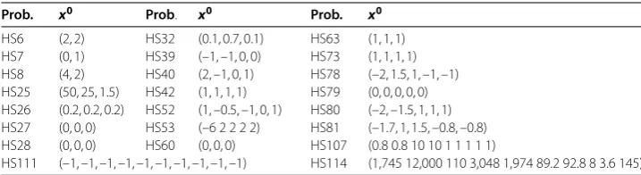
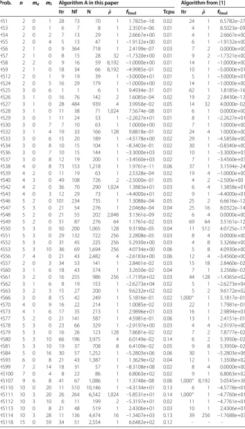
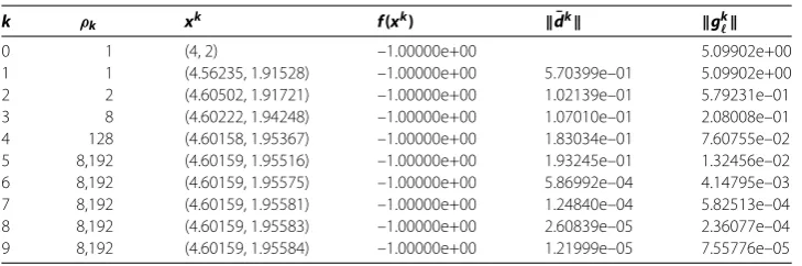
5 Numerical experiments
In this section, to show the practical effectiveness of Algorithm A, we test typical prob-lems from []. The numerical experiments are implemented by using MATLAB Ra, and on a PC with Inter(R) Core(TM) i- . GHz CPU, . GB RAM. The details about the implementation are described as follows.
5.1 Computing matrixHk
During the process of iteration, to ensure the boundedness of{Hk}, by modifying the com-puting technique in [] for the approximate Lagrangian Hessian, we introduce a slightly new computing method for the approximate Hessian matrixHkin Step as follows from second order derivative information. Denote vectorzˆkand matrixMkby
ˆ
zk=zkI,zkIı k, I
ı\Iı k
, ()
Mk=∇xxLρk
xk,zˆk– j∈I
ˆ zkj
gkj∇g
k j∇gk
T
j . ()
Then compute the smallest eigenvalueϑmink of matrixMk, and yield
θk= ⎧ ⎪ ⎪ ⎨ ⎪ ⎪ ⎩
, ifϑk
min>ε;
–ϑk
min+ε, if|ϑmink | ≤ε;
|ϑmink |, otherwise.
()
Subsequently, compute matrixHkin Step by
Hk= ⎧ ⎨ ⎩
∇
xxLρk(xk,zˆk) +θkEn, ifρk≤εandθk≤ε;
En, otherwise,
()
where the positive parametersεandεsame as the ones in Algorithm A are sufficiently small and sufficiently large, respectively.
The sequence{Hk}of matrices defined above possesses nice properties as follows.
Theorem Suppose thatX˜ =∅and assumptionsHandH(i)hold.Yield matrix Hk
in Stepby()-().If the sequence{xk}yielded by Algorithm Ais bounded, then the
following results hold.
(i) The sequence{Hk}is bounded and satisfies the positive definite restriction()with
constanta=ε,soHholds.
(ii) In addition,assume thatH(ii)and()are satisfied.Then,forklarge enough,
matrixMkis positive definite,ϑmink > andθk<ε.Therefore,Hkis always yielded
by the first case in(),i.e.,
Hk=∇xxLρk