2018 IX International Conference on Optimization and Applications (OPTIMA 2018) ISBN: 978-1-60595-587-2
The Lemke–Howson Algorithm Solving Finite Non-Cooperative
Three-Person Games in a Special Setting
Evgeny Golshteyn
1, Ustav Malkov
1, and Nikolay Sokolov
1Central Economics and Mathematics Institute of Russian Academy of Science, Nakhimovsky Prospect 32 117418 Moscow, Russia
[email protected], sokolov [email protected]
Bimatrix game, Hexamatrix game, Function, Mixed strategies, Nash equilibrium, Lemke– Howson algorithm
Abstract. We present a brief outline of an approximate method (3LP) proposed by E.G. Gol-
shteyn for solving three-person games in mixed strategies. Similar to the 2LP-algorithm (which approximately solves bimatrix games), the solution procedure consists in the search of a global minimum of the so-called Nash function. By making an exhaustive search of the pairs of the initial strategies the algorithm 2LP (3LP) finds an exact solution of the game if the condition of recip- rocal complementarity holds. The numerical experiments show that the 2LP-method successfully competes with the Lemke–Howson (LH) algorithm, which efficiently solves the bimatrix games. Unfortunately, the LH-algorithm cannot be applied to solve arbitrary three-person games. How- ever, we have adapted the Lemke–Howson method to the solution of a special setting called the hexamatrix games. We have also conducted a thorough testing of the LH-algorithm to reveal its advantages and minor points as well.
Introduction
In [1] an algorithm approximately solving finite non-cooperative three-person games (3LP) was proposed. The testing results illustrating the efficiency of the said method’s application can be found in [2]. In this paper, we have tested the 3LP-algorithm as applied to a special setting of the 3-persons game [7]. Moreover, we have managed to adapt the classical Lemke–Howson (LH) method [4] to the solution of the 3-persons game in the above-mentioned special setting. Let us specify both the general and the special settings of the 3-persons games.
The Three-Person Game in the General Setting
A finite non-cooperative 3-persons game Γ is defined with three sets X, Y, Z of strategies of the first, second, and third player respectively, where X = {x = (x1, . . . , xm)T ∈ Em : xTem = 1, x om}, Y = {y = (y1, . . . , yn)T ∈ En : yTen = 1, y on}, Z = {z = (z1, . . . , zl)T ∈ El : zTel = 1,
1
Keywords:
z >ol}, together with their payoff functions as follows
fx(ω) = m
X
i=1 n
X
j=1 l
X
k=1
aijkxiyjzk,
fy(ω) = m
X
i=1 n
X
j=1 l
X
k=1
bijkxiyjzk,
fz(ω) = m
X
i=1 n
X
j=1 l
X
k=1
cijkxiyjzk.
Here, one has (aijk), (bijk), (cijk) — the players’ 3-dimensional payoff tables (without any loss of
generality one can assume that all the entries of those tables are positive real numbers), dijk :=
aijk +bijk +cijk (1 6 i 6 m, 1 6 j 6 n, 1 6 k 6 l); the vector ωT = (xT, yT, zT), ω ∈
Ω = X ×Y ×Z ⊂ Em++n+l. Next, for p = m, n, l, we define the vectors op = (0, . . . ,0)T ∈ Ep+, ep = (1, . . . ,1)T ∈ Ep, as well as Ep+ — the nonnegative orthant of the Euclidean space Ep. The
symbol T denotes the operation of transposition of a vector (matrix).
Introduce the Nash function (indicator): F(ω) = δx(ω) +δy(ω) +δz(ω), where
δx(ω) = max x0∈X fx(x
0
, y, z)−fx(ω),
δy(ω) = max
y0∈Y fy(x, y
0
, z)−fy(ω),
δz(ω) = max
z0∈Z fz(x, y, z
0
)−fz(ω).
The function F(ω) is an analogue of the Nash function defined for the bi-matrix games [5]. As the above-defined payoff functions are linear with respect to each variable x, y, z (when the other two variables are fixed), the game Γ is convex, hence the set of Nash points Ω∗ is non-empty (but not necessarily convex). For the definition of the convex games and their properties the reader is referred to [6].
Since F(ω) > 0 for all ω ∈ Ω, and F(ω) = 0 if, and only if ω is the (equilibrium) point of the game Γ, one can find the solution of game Γ as the global minimum (equalling zero) of the function F(ω) on Ω.
The 3LP-Method for Solving the 3-Persons Game in the General Setting
Set the iteration counter t = 0. As an initial (starting) strategy, one can use any pair of the players’ pure strategies (the total number of such pairs is mn+ml+nl); for example, fix a pair of strategies {y(0), z(0)} with the components y(0)
1 = 1, y (0)
j = 0, j = 2, . . . , n, z (0) 1 = 1, zk(0) = 0, k = 2, . . . , l, and solve successively (fort= 0,1, . . .) the triple problemPx(y(t), z(t);x(t+1)),
Py(x(t+1), z(t);y(t+1)), andPz(x(t+1), y(t+1);z(t+1)), where
Px(y0, z0;x) : m X i=1 n X j=1 l X k=1
dijkyj0z
0
k
xi−β−γ −→max x,β,γ, m X i=1 l X k=1 bijkzk0
xi−β 60, j = 1, . . . , n,
m X i=1 n X j=1 cijky0j
xi−γ 60, k= 1, . . . , l,
xTem = 1, x>om, β, γ ∈E1+.
If x∗ is an optimal solution of this problem, then we setx0 :=x∗; next we solve:
Py(x0, z0;y) : n X j=1 m X i=1 l X k=1
dijkx0iz
0
k
yj −α−γ −→max y,α,γ, n X j=1 l X k=1 aijkz0k
yj −α60, i= 1, . . . , m,
n X j=1 m X i=1 cijkx0i
yj−γ 60, k = 1, . . . , l,
yTe
n= 1, y>on, α, γ ∈E1+.
Again, if y∗ is an optimal plan for the above problem, then put y0 :=y∗, and continue solving:
Pz(x0, y0;z) : l X k=1 m X i=1 n X j=1
dijkx0iy
0
j
zk−α−β −→max z,α,β, l X k=1 m X i=1 bijkx0i
zk−α60, j = 1, . . . , n,
l X k=1 n X j=1 cijky0j
zk−β 60, i= 1, . . . , l,
zTe
l = 1, z >ol, α, β ∈E1+.
Now that z∗ is an optimal solution of that problem, we denotez0 :=z∗.
The optimal objective function values Ft ≡F(ω(t+1)) are monotone non-increasing by t. The
iteration process continues until the valueFtstabilizes, that is, for somet∗, the differenceFt∗−Ft∗+1
becomes small enough. In addition, ifFt∗ = 0, it means that an (exact) Nash point has been found.
If the value Ft∗ is positive but small enough, an approximate solution of the game is reported.
Otherwise, select a new pair of the initial strategies and start the process again (probably, having altered the order of the solved problems Px, Py, Pz).
The 3-Persons Game in a Special Setting: the Hexamatrix Game
We propose this special setting of the 3-persons game in order to check the efficiency of the 3LP-method as applied to such particular cases, as well as to develop a new algorithm inapplicable for the games in the general form but quite reliable when solving the special games.
Consider the set of hexamatrix games (i.e., the poly-matrix 3-persons games) introduced by A.S. Strekalovsky [7]. A hexamatrix game is defined by 6 matrices:
A1 = (a1ij), A2 = (a2ik), B1 = (b1ji), B2 = (b2jk), C1 = (c1ki), C2 = (c2kj),
with the players’ payoff functions of the form
fx(ω) = xT(A1y+A2z), fy(ω) = yT(B1Tx+B2z), fz(ω) =zT(C1Tx+C2Ty).
The 3LP-Algorithm Solving Hexamatrix Games
In order to solve a hexamatrix game Γ one needs to solve the quadratic programming problem:
P :
xT(A1y+A2z) +yT(B1Tx+B2z) +zT(C1Tx+C2Ty)−α−β−γ −→ max ω,α,β,γ,
A1y+A2z 6αem, B1Tx+B2z 6βen, C1Tx+C2Ty6γel,
xTem = 1, x>om, yTen = 1, y>on, zTel = 1, z >ol, α, β, γ ∈E1+.
The hexamatrix game can be solved by the same 3LP-method if one replaces the above-listed formulas Px(y0, z0;x0),Py(x0, z0;y0) and Pz(x0, y0;z0) with the following ones:
Px(y0, z0;x) :
xT(A1y0 +A2z0 +BT1y 0
+C1Tz0) + (y0)TB2z0+ (z0)TC2Ty 0−
β−γ −→max
x,β,γ,
BT
1x6βen−B2z0, C1Tx6γel−C2Ty
0, xTe
m = 1, x>om, β, γ ∈E1+, Py(x0, z0;y) :
yT(B1Tx0+B2z0 +AT1x 0
+C2Tz0) + (x0)TA2z0 + (z0)TC1Tx 0−
α−γ −→max
y,α,γ,
A1y 6αem−A2z0, C2Ty 6γel−C1Tx
0, yTe
n=l, y>on, α, γ ∈E1+, Pz(x0, y0;z) :
zT(C1Tx0+C2Ty0 +AT2x0+B2y0) + (x0)TA1y0+ (y0)TB1Tx 0−
α−β −→max
z,α,β,
B2z 6βen−B1Tx 0, A
2z 6αem−A1y0, zTel = 1, z >ol, α, β ∈E1+.
The LH-Algorithm Solving the Hexamatrix Game
The Lemke–Howson (LH) algorithm finds the solution of a game by solving the system of linear constraints in the linear complementarity problem associated with the game in question. The LH-method has been described in the paper [3], in which we compared the efficiency of this algorithm with the 2LP-method of finding Nash points of bimatrix games. In more detail, in the case of a bi-matrix game, the LH-algorithm first applies the linear transformation of variables
x0 = x/α, y0 = y/β to obtain the linear complementarity problem tantamount to the original problem. However, in the case of the 3-persons game in the special setting such a transformation fails. Nevertheless, we can generate a series of auxiliary problems (see below) and solve them by the LH-method to find a Nash point.
As the 3-persons game Q in the special setting stated below
Q: A1y+A2z+u=αem, B1Tx+B2z+v =βen, C1Tx+C2Ty+w=γel,
xTem = 1, yTen= 1, zTel = 1,
x, u∈Em+, y, v∈En+, z, w∈El+, α, β, γ >0,
has all linear constraints, one is inclined to try to solve it with the Lemke–Howson algorithm as a bi-matrix game. However, in contrast to a bi-matrix game, here we have to solve an auxiliary problem in order to generate a starting point.
Namely, the following complementarity conditions must be valid at any Nash equilibrium point:
xiui = 0, 16i6m, yjvj = 0, 16j 6n, zkwk= 0, 16k6l.
Having set α= 1, β = 1, γ = 1,we reduce the auxiliary problem to the equations system
A1y+A2z+u=em, B1x+B2z+v =en, C1x+C2y+w=el,
x, u∈Em+, y, v∈En+y, z, w ∈El.‘
Now introduce the notation: q =m+n+l,
H =
Om A1 A2 B1 On B2 C1 C2 Ol
, s =
x y z
, σ =
u v w
,
e=eq,
o=oq,
E = diag (e),
where for p=m, n, l, all elements of the square matrix Op of dimension p are zero, E is the unit
matrix of dimension q, we generate the following complementarity problem: Find a nonnegative solution (s, σ >0) to the linear system Hs+ Eσ =e. In order to solve the latter problem, make use of a procedure of Lemke–Howson type. Namely, select σ as an initial basis. Introduce the variable x1 into the basis. As a result, another variable leaves the basis without breaking the
nonnegativity of the basic variables. Next, the variable related to the leaving basic variable in the complementarity condition is introduced into the basis. This operation is repeated until the variable x1 leaves the basis. The result will be a “pseudo-Nash” point. As the Lemke–Howson
procedure may suffer looping, we impose an additional restriction: after starting from a current initial point, we admit only a fixed (bounded) number of iterations, e.g., not exceeding q (which is the game’s dimension). Here, the term “Nash pseudo-equilibrium” is cited in quotes, because when solving the auxiliary system we relaxed (didn’t include) the restrictionsxTe
m = 1, yTen = 1,
zTe l = 1.
The starting points are selected successively, in the order of the components of the vector s:
x1, . . . , xm, y1, . . . , yn, z1, . . . , zl (n+m+l in total). The thus generated basis is used as an initial
basis for the problem Q. The latter is constructed in the following manner. First, we introduce into the basis the basic variables of the auxiliary problem and put them into the same positions that they occupied in the basis of the auxiliary problem. Sure there will be some variables that are impossible to introduce into the basis in their own positions because the leading coefficients of the decompositions of the corresponding columns with the respect to the current basis might be very close to zero. Those variables are introduced into the basis in the yet occupied positions but such that the leading coefficients have large enough absolute values. The solution thus generated may contain negative basic values. In the latter case, we repeat the solution of the auxiliary problem starting from the next initial point. The obtained solution with nonnegative basic values has the same structure as the solution of the auxiliary problem, that is, it satisfies the complementarity conditions, and hence is a Nash point.
The conducted tests demonstrated that a relatively moderate number of “pseudo-Nash” points was necessary to generate before obtaining the final solution.
Test Results for the 3LP- and LH-Algorithms
We tested the algorithms solving the 3-persons games in both the general and the special settings by making use of the personal computer with the processor Intel(R) Core(TM) i5-3427U CPU @ 1.80GHz 2.300 GHz, memory 4.00 GB, 4 cores). The test codes were written in the languages FORTRAN, MatLab, and Python. A series of S games was solved for each triple
n, m, l.
The matrices were generated in two stages. For the games in the general setting, we first used a pseudo-random counters to generate independently the elements of the auxiliary tables
a0ijk, b0ijk, c0ijk (1 6 i 6 m, 1 6 j 6 n, 1 6 k 6 l); at the second stage, we constructed the payoff tables by the formulas
aijk =a0ijk+κ(b
0
ijk+c
0
ijk), bijk =b0ijk+κ(a
0
ijk+c
0
ijk), cijk =c0ijk+κ(a
0
Ijk+b
0
ijk)
for all i, j, k. Hereκ is the coefficient of reciprocal dependence of the payoff tables, 06κ 61/2. For the games in the special setting, this procedure can be made only when n=m=l. In the latter case, we first generated independently the pseudo-random matrices A01, A02, B10, B20, C10, C20, then produced the payoff matrices as follows:
Ai =A0i+κ(B
0
i +C
0
i), Bi =Bi0+κ(A
0
i+C
0
i), Ci =Ci0 +κ(A
0
i+B
0
i), i= 1,2.
If the sizes n, m, l are the same, then the games generated in those two settings are different and are solved differently, too. In the case of the general setting, one can solve games up to the dimension n = m= l = 350, while in the case of the special setting — up to 2000. However, the 3LP-method may fail by requiring an unacceptable computational time.
The upper part of Table 1 reports the results of the LH-algorithm solving the set of test games (5 series with 10 instances in each) in the general setting with independent matrices (κ = 0). The algorithm switched to the next initial pair of strategies after having made dim iterations.
In the lower part of Table 1, the initial pair of strategies were changed after dim/4 iterations passed by the LH-algorithm. The two bottom lines of the table report the results of solving a game of dimensions n = m = l = 500 and with dependent payoff matrices (the reciprocal dependence coefficient (κ) equals 0.1 and 0.2, respectively).
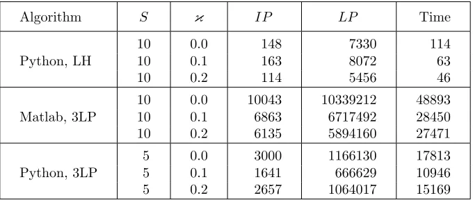
Here in Table 1 and onward, the following notation is used: n, m, l are the game’s sizes,
dim = n +m +l — the game’s dimension; S —the number of games in each series; κ — the coefficient of the reciprocal dependence of the payoff matrices;IP — the total number of the used initial starting strategies; LP — the total number of the simplex-type steps; Time — the total amount of time to solve S games (sec); neg — the total number of Nash pseudo-equilibria with negative basic values in the basis generated for the original problem/game.
Is easy to see from the reported results (see the last three rows in table 1.), the reciprocal dependence of the payoff matrices doesn’t affect much or even decreases the computational efforts to solve a problem in the special setting by the LH-algorithm. However, for the general setting and the 3LP-algorithm, the situation was different. The reciprocal dependence sufficiently increases the complexity of problems. Such results were produced and reported in detail in our previous paper [2]. For example, on the one hand, when solving the series of 10 problems 100x100x100 with independent matrices the result was yielded in 276 sec by making use of 48 initial points. On the other hand, when the matrices were reciprocally dependent (κ= 0.1) we had to use 15440 starting points in order to finish in 78816 sec.
Table 1. The LH-algorithm solving the family of 50 three-person games in the special setting
n=m=l S κ IP LP Time neg
100 10 0.0 101 5812 123 16 200 10 0.0 261 21732 1155 16 dim 300 10 0.0 551 77394 5188 16 400 10 0.0 902 131059 21428 28 500 10 0.0 1456 120947 57013 28
100 10 0.0 447 7408 177 16 200 10 0.0 668 16510 864 16 300 10 0.0 1074 35424 3261 16 dim/4 400 10 0.0 1144 77157 6020 28 500 10 0.0 2464 104020 27015 28 500 10 0.1 756 44334 8394 28 500 10 0.2 1406 41064 14195 28
Table 2. The results of solving the game 100×100×100 in the special s setting by the LH- and 3LP-algorithms
Algorithm S κ IP LP Time
10 0.0 148 7330 114 Python, LH 10 0.1 163 8072 63
10 0.2 114 5456 46
10 0.0 10043 10339212 48893 Matlab, 3LP 10 0.1 6863 6717492 28450 10 0.2 6135 5894160 27471
5 0.0 3000 1166130 17813 Python, 3LP 5 0.1 1641 666629 10946 5 0.2 2657 1064017 15169
Conclusions
The realized theoretical research and numerical experiments allow one to evaluate the compu-tational efficiency of the 3LP- and LH-algorithms, as well as to discover their strong and minor points.
We have successfully adapted the Lemke–Howson method to the solution of 3-persons games in the special setting: hexamatrix games. All the tested examples have been solved by making use of essentially smaller numbers of initial strategies and much lower computational time than the 3LP-algorithm.
References
[1] E. Golshtein. A Numerical Method for Solving Finite Three-Person Games, Economica i Matematicheskie Metody 50(1) (2014) 110–116 (In Russian).
[image:7.612.137.477.370.514.2][2] E. Golshtein, U. Malkov, and N. Sokolov. Efficiency of an Approximate Algorithm to Solve Finite Three-Person Games (a Computational Experience), Economica i Matematicheskie Metody, 53(1)(2017) 94–107 (In Russian).
[3] E. Golshtein, U. Malkov, and N. Sokolov. On a Numerical Method for Solving Bimatrix Games, Economica i Matematicheskie Metody 49(4) (2013) 94–104 (In Russian).
[4] C. Lemke and CJ Howson. Equilibrium Points of Bimatrix Games, Journal of the Society for Industrial andApplied Mathematics 12 (1964) 778–780.
[5] H Mills. Equillibrium Points in Finite Games, Journal of the Society for Industrial and Applied Mathematics 8(2) (1960) 397–402.
[6] M Osborne. An Introduction to Games Theory, New-York: Oxford University Press (2004). [7] A Strekalovsky and R Enkhbat. Polymatrix Games and Optimization Problems,AvtomatikaI
Telemekhanika (4) (2014) 51–66.