Bubbles and crashes in finance: A phase transition from random to deterministic behaviour in prices

Munich Personal RePEc Archive

Bubbles and crashes in finance: A phase

transition from random to deterministic

behaviour in prices.

Fry, J. M.

university of east london

3 September 2010

Online at

https://mpra.ub.uni-muenchen.de/24778/

Bubbles and crashes in finance: A phase

transition from random to deterministic

behaviour in prices

John M. Fry

September 2010

Abstract

We develop a rational expectations model of financial bubbles and study ways in which a generic risk-return interplay is incorporated into prices. We retain the interpretation of the leading Johansen-Ledoit-Sornette model, namely, that the price must rise prior to a crash in order to compensate a representative investor for the level of risk. This is accompanied, in our stochastic model, by an illusion of certainty as described by a decreasing volatility function. As the volatility function goes to zero, crashes can be seen to represent a phase transition from stochastic to deterministic behaviour in prices.

Keywords: financial crashes, super-exponential growth, illusion of certainty, housing-bubble.

1

Introduction

Rational expectations models were introduced with the work of Blanchard and Watson to account for the possibility that prices may deviate from fundamental levels [1]. We take as our main starting point the somewhat controversial subject of log-periodic precursors to financial crashes [2]-[11], with a fundamental aim of our approach being relatively easy

∗_{UEL Royal Docks Business School, Docklands Campus, University of East London, London E16 2RD}

calibration of our model to empirical data. Additional background on log-periodicity and complex exponents can be found in [12]. A first-order approach in [3] and subsequent extensions in [13] state that prior to a crash the price must exhibit a super-exponential growth in order to compensate a representative investor for the level of risk. However, this approach concentrates solely on the drift function and ignores the underlying volatility fluctuations which typically dominate financial time series [14]. Similar in spirit to [3], we derive a second-order condition which incorporates volatility fluctuations and enables us to combine insights from a rational expectations model with a stochastic model [15]-[16].

Our model gives two important characterisations of bubbles in economics. Firstly, a rapid super-exponential growth in prices. Secondly, an illusion of certainty as described by a decreasing volatility function prior to the crash. As the volatility function goes to zero bubbles and crashes can be seen to represent a phase transition from stochastic to purely deterministic behaviour in prices. This clarifies the oft cited link in the literature between phase transitions in critical phenomena and financial crashes. Further, this recreates the phenomenology of the Sornette-Johansen paradigm: namely that prices resemble a deterministic function prior to a crash. We explore a number of different applications of our model and the potential relevance to recent events is striking.

The layout of this paper is as follows. In Section 2 we introduce the basic model and derive the crash-size distribution, the post-crash dynamics, simple estimates of fundamental-value and speculative-bubble components. Section 3 describes an empirical application to the UK housing bubble of the early to late 2000s [17]. Section 4 is a brief conclusion.

2

The model

In this section we give an alternative formulation of the model solution in [3]. This leads naturally to a stochastic generalisation of the original model, which is then solved in full to give empirical predictions for the distribution of crash-sizes, post-crash dynamics, fundamental values and the level of over-pricing.

We offer an alternate derivation of the basic model in [3] as follows. Let P(t) denote

the price of an asset at time t. Our starting point is the equation

where P1(t) satisfies

dP1(t) =µ(t)P1(t)dt+σ(t)P1(t)dWt, (2)

where Wt is a Wiener process and j(t) is a jump process satisfying

j(t) = (

0 before the crash

1 after the crash. (3)

When a crash occurs κ% is automatically wiped off the value of the asset. Prior to a

crash P(t) =P1(t) and Xt = log(P(t)) satisfies

dXt= ˜µ(t)dt+σ(t)dWt+ ln[(1−κ)]dj(t), (4)

where ˜µ=µ(t)−σ2_{(t)/2. If a crash has not occurred by time t, we have that}

E[j(t+δ)−j(t)] = h(t)dt+o(dt), (5)

Var[j(t+δ)−j(t)] = h(t)dt+o(dt), (6)

whereh(t) is the hazard rate. We compare (4) with the prototypical Black-Scholes model

for a stock price:

dXt =µdt+σdWt, (7)

and use (7) as our model for “fundamental” or purely stochastic behaviour in prices.

The first-order condition see e.g. [1], [3], suggests that ˜µ(t) in (4) grows in order

to compensate a representative investor for the risk associated with a crash. The

instantaneous drift associated with (4) is

˜

µ(t) + (ln(1−κ))h(t). (8)

For (7) the instantaneous drift is µ. Setting (8) equal to µ, it follows that in order for

bubbles and non-bubbles to co-exist

˜

µ(t) =µ−(ln(1−κ))h(t). (9)

If we ignore volatility fluctuations by setting σ(t) = σ, then our pre-crash model for an

asset price becomes

However, this is actually a rather poor empirical model [18], failing to adequately account for the volatility fluctuations in (4). Under a Markowitz interpretation, means represent

returns and variances/standard deviations represent risk. Suppose that in (4)σ(t) adapts

in an analogous way to µ(t) so as to compensate a representative investor for bearing

additional levels of risk. The instantaneous variance associated with (4) is

σ2(t) + (ln(1−κ))2h(t). (11)

For (7) the instantaneous variance is σ2_{. Setting (11) equal to σ}2_{, the second-order}

condition for co-existence of bubbles and non-bubbles becomes

σ2_{(t) = σ}2_{−(ln(1−κ))}2_{h(t). (12)}

(12) illustrates an illusion of certainty – a decrease in the volatility function – which

arises as part of a bubble process. Intuitively, in order for a bubble to occur not only must returns increase but the volatility must also decrease. If this does not happen (7)

with an instantaneous variance of σ2 _{would represent a more attractive and less risky}

investment than a market described by (10) and bubbles could not occur. We use (7) as a model of a ‘fundamental’ or purely stochastic regime, as in Black-Scholes theory. From (12), our model for prices under a bubble regime becomes

dXt= [µ−ln(1−κ)h(t)]dt+pσ2_{−(ln(1−κ))}2_{h(t)dWt. (13)}

The simplest h(t) considered in [3] is

h(t) = B(tc−t)−α, (14)

where it is assumed that α ∈ (0,1) and tc is a critical time when the hazard function

becomes singular, by analogy with phase transitions in statistical mechanical systems [19]. Here, we choose on purely statistical grounds

h(t) = βt

β−1

αβ_+tβ, (15)

which is the form corresponding to a log-logistic distribution and is intended to capture the essence of the previous approach as the hazard rate has both a relatively simple form

and, forβ >1, has a non-trivial mode at t=α(β−1)β1, with modal point (β−1)1−β1/α.

log-logistic distribution has probability density

f(x) = βα

β_xβ−1

(αβ _+xβ₎2, (16)

on the positive half-line. The cumulative distribution function is

F(x) = 1− α

β

αβ _+xβ (17)

The model (13) with h(t) given by (15) has the solution

Xt=X0+µt+vln

µ

1 + t

β αβ ¶ + Z t 0 r

σ2_−v2 βtβ−1

αβ_+tβdWu. (18)

where v =−ln(1−κ) withv >0. From (18) the conditional densities can be written as

Xt|Xs∼N(µt|s, σt2|s), (19)

where

µt|s = Xs+µ(t−s) +vln

µ

αβ_+tβ αβ_+sβ

¶

, (20)

σ_t2_|s = σ2(t−s)−v2ln µ

αβ_+tβ αβ_+sβ

¶

. (21)

Under the fundamental equation (7) these expressions are simplyµt|s =Xs+µ(t−s) and

σ2

t|s =σ2(t−s). Thus, we see that under the bubble model the incremental distributions

demonstrate a richer behaviour over time.

The fundamental or purely stochastic non-bubble model (7) corresponds to the case

that κ = 0, or equivalently that v = 0. We can test for bubbles by testing the null

hypothesis v = 0 (no bubble) against the alternative hypothesis v > 0 (bubble). This

can be simply done using a (one-sided) t-test since maximum likelihood estimates, and

estimated standard errors, can be easily calculated numerically from (19). A range of further implications of our bubble model can be derived as we describe below.

Crash-size distribution. Suppose that prices are observed up to and including timetand

that a crash has not occurred by time t. The crash-size distribution resists an analytical

description but a Monte Carlo algorithm to simulate the crash-size C is straightforward

and reads as follows:

1. Generate u fromU ∼Log-logistic(α, β) with the constraintu≥t.

where

Z∼N

µ

Xt+µu+vln µ

αβ_+uβ αβ_+tβ

¶

, σ2u−v2ln µ

αβ_+uβ αβ_+tβ

¶¶

(22)

We note that simulating ufrom the log-logistic distribution is straight-forward and from

(17) possible via inversion using

F−1(x) = α

µ

x

1−x

¶_β1

or F−1(x) =

µ

αβ_+tβ

1−x −α

β

¶β1

with constraint u≥t.

Post-crash increase in volatility. Before a crash equation (18) applies. After a crash, the price reverts to the fundamental price dynamics (7). Suppose the crash occurs at time

C. At t=C we have that

Var(Xt+h|Xt) =σ2h, (23)

but for t < C

Var(Xt+h|Xt) =σ2h−v2ln

µ

αβ _{+ (t+h)}β αβ _{+ (t)}β

¶

(24)

Thus, our model predicts an increase in volatility following a crash given by

κ2ln µ

αβ_{+ (t+h)}β αβ_{+ (t)}β

¶

. (25)

Fundamental values. The above model suggests a simple approach to estimate

fundamental value. Under the fundamental dynamics (7)

PF(t) := E(P(t)) =P(0)eµt, (26)

and we use (26) to estimate fundamental value in our empirical application in Section 7. This approach recreates the widespread phenomenology of approximate exponential growth in economic time series (see e.g. Chapter 7 in [21]).

Estimated bubble component.Define

H(t) = Z t

0

h(u)du. (27)

Xt= log(Pt) satisfies

Xt ∼N¡

X0+ ˜µt+vH(t), σ2t−v2H(t)

¢

, (28)

it follows that

PB(t) :=E(P(t)) =P(0)eµt+

³

v−v2

2

´

H(t)

. (29)

This motivates the following estimate for the proportion of observed prices which can be attributed to a speculative bubble:

1− 1

T

Z T

0

PF(t)

PB(t) dt = 1− 1

T

Z T

0

µ

1 + t

β

αβ

¶−(v−v2/2)

dt. (30)

3

Empirical application

As an empirical application we consider the UK housing bubble from 2002-2007 by modelling a monthly time series of average UK house prices. The null hypothesis of

no bubble is a test of the hypothesis v = 0. This can be tested using a one-sided t-test

– dividing the estimate ˆv by its estimated standard error and comparing to a normal

distribution. For this data set we obtain a t-statistic of 3.66 and a p value of 0.0001 to

give strong evidence of a bubble in this data.

From our fit of the bubble model (18) we use PF(t) = P(0)eµt _{in (26) as a simple}

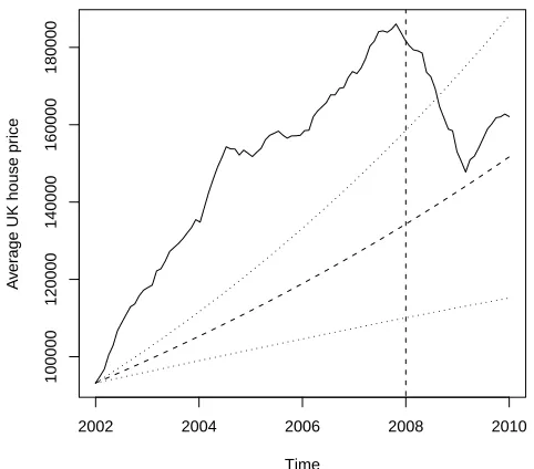
estimate of fundamental value. A plot of UK house prices together with estimated fundamental values and associated 95% confidence intervals is shown in Figure 1. Prices appear to be well in excess of fundamental values, with prices lying above the upper confidence limits of the estimated fundamental values throughout the sample (Figure 1 to the left of the vertical line). We then estimate fundamental value for the years 2008-2009 using data from 2002-2007 only and compare with the actual historically observed

prices. That is, we use our model to provide estimates of fundamental value out of

2002 2004 2006 2008 2010

100000

120000

140000

160000

180000

Time

A

v

er

age UK house pr

ice

Figure 1: Plot of average UK house-prices and estimated fundamental value (dashed line) and associated 95% confidence intervals (dots). Estimation takes place over the period 2002-2007 (to the left of the dashed vertical line). Out-of-sample estimates of fundamental value are then compared to historically observed prices (to the right of the dashed vertical line).

4

Conclusions

References

[1] Sornette, D. and Malevergne, Y. (2001) From rational bubbles to crashes Physica A

299 40-59.

[2] Sornette, D. and Johansen, A., (1997) Large financial crashes Physica A, 245,

411-422.

[3] Johansen, A., Ledoit, O. and Sornette, D. (2000) Crashes as critical points Int. J.

Theor. and Appl. Finan.,3, 219-255.

[4] Johansen, A. (2004) Origins of crashes in 3 US stock markets: shocks and bubbles Physica A. 338 135-142.

[5] Laloux, L., Potters, M., Cont, R., Aguilar, J.-P and Bouchaud, J.-P. (1999) Are

financial crashes predictable? Europhys Lett. 45 1-5.

[6] Johansen, A. (2002) Comment on “Are financial crashes predictable?”Europhys Lett.

60 809-810.

[7] Feigenbaum, J. A. and Freund, P. G. O. (1996) Discrete scale invariance in stock

markets before crashes Int. J. Mod. Phys. B 10 346-360.

[8] Feigenbaum, J. A. (2001a) A statistical analysis of log-periodic precursors to financial

crashes Quant. Finan.1 346-360.

[9] Feigenbaum, J. (2001b) More on a statistical analysis of log-periodic precursors to

financial crashes Quant. Finan.1 527-532.

[10] Chang, G., and Feigenbaum, J. (2006) A Bayesian analysis of log-periodic precursors

to financial crashesQuant. Finan. 6 15-36.

[11] Chang, G., and Feigenbaum, J. (2008) Detecting log-periodicity in a regime-switching

model of stock returns Quant. Finan. 8 723-738.

[12] Sornette, D. (1998) Discrete scale invariance and complex dimensions Phys. Reps

297 239-270.

[13] Zhou, W-X. and Sornette, D. (2006) Fundamental factors versus herding in the

2002-2005 US stock market and prediction Physica A 360 459-482.

[14] Cont, R. and Tankov, P. Financial modelling with jump processes. Chapman and

[15] Sornette, D. and Andersen, J-V. (2002) A nonlinear super-exponential rational model

of speculative financial bubbles. Int. J. Mod. Phys. C 17 171-188.

[16] Andersen, J-V., and Sornette, D. (2004) Fearless versus fearful speculative financial

bubbles. Physica A, 337 565-585.

[17] Zhou, W-X. and Sornette, D. (2003) 2000-2003 real estate bubble in the UK but not

in the USA Physica A329 249-262.

[18] Fry, J. M. (2008) Statistical modelling of financial crashes PhD thesis, Department

of Probability and Statistics, University of Sheffield.

[19] Yeomans, J. M. (1992) Statistical mechanics of phase transitions, Oxford University

Press.

[20] Cox, D. R. and Oakes, D. (1984)Analysis of survival data. Chapman and Hall/CRC,

Boca Raton London New York Washington, D. C.

[21] Campbell, J. Y., Lo., A., and MacKinlay, J. A. C. (1997) The econometrics of

financial markets, Princeton University Press, Princeton.

[22] Black, A., Fraser, P., and Hoseli, M. (2006) House prices, fundamentals and bubbles J. Bus. Fin. and Account. 33 1535-1555.

[23] Hott, C. and Monnin, P. (2008) Fundamental real estate prices: An empirical

estimation with international data, Journal of Real Estate and Financial Economics