Prediction of Sewer Pipe Main Condition Using the Linear Regression Approach

http://dx.doi.org/10.4236/gep.2016.45010

Prediction of Sewer Pipe Main Condition

Using the Linear Regression Approach

1_{Ladhane Consultant Engineering, Roorkee, India}

2_{Civil Engineering Department, University of Roorkee, Roorkee, India}

Received 16 March 2016; accepted 16 May 2016; published 19 May 2016

Copyright © 2016 by authors and Scientific Research Publishing Inc.

This work is licensed under the Creative Commons Attribution International License (CC BY). http://creativecommons.org/licenses/by/4.0/

Abstract

This research presents the condition prediction of sewer pipes using a linear regression approach. The analysis is based on data obtained via Closed Circuit Television (CCTV) inspection over a sew-er system. Information such as pipe matsew-erial and pipe age is collected. The regression approach is developed to evaluate factors which are important and predict the condition using available in-formation. The analysis reveals that the method can be successfully used to predict pipe condition. The specific model obtained can be used to assess the pipes for the given sewer system. For other sewer systems, the method can be directly applied to predict the condition. The results from this research are able to assist municipalities to forecast the condition of sewer pipe mains in an effort to schedule inspection, allocate budget and make decisions.

Keywords

Sewer Pipe Main, Rehabilitation, Regression, Condition Prediction, Deterioration

1. Introduction

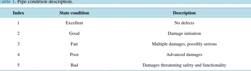
The pipe conditions are obtained via various approaches. Some of available inspection techniques include: man-walk though, ultrasonic, focused electrode leak location (FELL), sewer scanner and evaluation technology (SSET), laser-based scanning system, and CCTV. The most popular method is the CCTV application. For the data used in this study, the condition data are primarily based on information obtained via CCTV. During the condition determination process, experts’ opinions are often adopted to rate a pipe section’s condition by com-bining all information. For the data used in this study, the pipe conditions are classified into 5 categories, as shown in Table 1.

Research regarding the sewer pipe condition deterioration has been widely studied in recent years. There are various models applied and developed in the condition prediction. For example, Moselhi and Shehab [2] classi-fied the defects in sewer pipes using the neutral networks. Ariaratnam et al. [3] assessed the infrastructure in-spection needs using logistic models. By using a set of condition data related to sewer pipes, they found that the model could be successfully used to predict system conditions. The most popular method used is the Markov chains model, which has been widely applied in the condition evaluation of all infrastructures. For example, Jin and Mukherjee [4] explored the Markov chain application in modeling facility deterioration by proposing mul-tiple methods to estimate the condition transition probabilities. They further evaluated the sensitivity of the model by using data obtained via simulations in Matlab. They concluded that the Markov model has very good robustness [5]. The findings were later applied in the life cycle analysis [6]. Similar studies regarding the Mar-kov chains model can also be found in [7]-[10]. Other studies related to sewer system include the failure analysis

[11]-[13]; and situational simulation to support decision making [14].

This study aims to evaluate the significance of variables related to sewer mains. It also tends to predict the pipe condition using the linear regression approach.

2. Methodology

The first step is the initial analysis of the data. The descriptive information includes pipe material, pipe diameter, pipe age, pipe installation depth. The pipe material includes concrete pipe and clay pipe. The pipe diameter ranges between 45 cm to 180 cm. The installation depth ranges between 65 cm to 213 cm. Additional data anal-ysis will be presented in the results section

The second step is the application of regression approach. The general linear model is a linear model specifies the relationship between a dependent variable Y, and as set of predictor variables Xi, therefore, we have

0 1 1 2 2 3 3

= + + + + + _{k k}

Y β β X β X β X  β X (1)

In the equation, β0 is the regression coefficient for the intercept and βi are the coefficients for the variable Xi. The βi values are obtained by the maximum likelihood (ML) estimation, which is an iterative computational procedure. There are multiple method for the Ml estimate, such as Newton-Raphson and Fisher-Scoring me-thods [15].

In terms of statistical significance testing, the test are usually performed via Wald statistic, the likelihood ratio (LR), or a score statistic. Detailed information can be found in McCullagh and Nelder [15]. In order to diagnose the linear model, the residuals are usually used to evaluate the fitting. There are two types of such residuals, Pearson residuals and deviance residuals [15]. The Pearson residuals are based on the difference between the observed data and the predicted values. The deviance residuals are related to the contribution of the observed data to the log-likelihood statistic [15].

Table 1.Pipe condition description.

Index State condition Description

1 Excellent No defects

2 Good Damage initiation

3 Fair Multiple damages, possibly serious

4 Poor Advanced damages

3. Results and Discussions

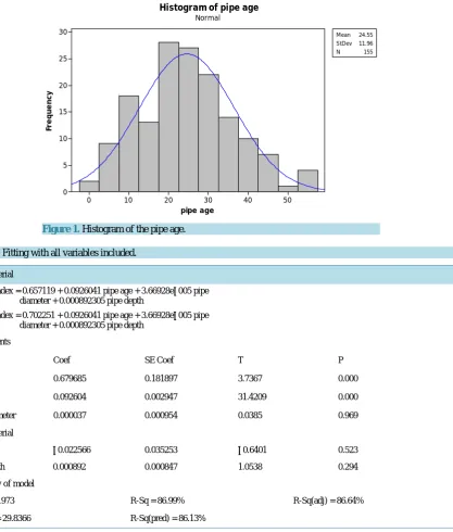
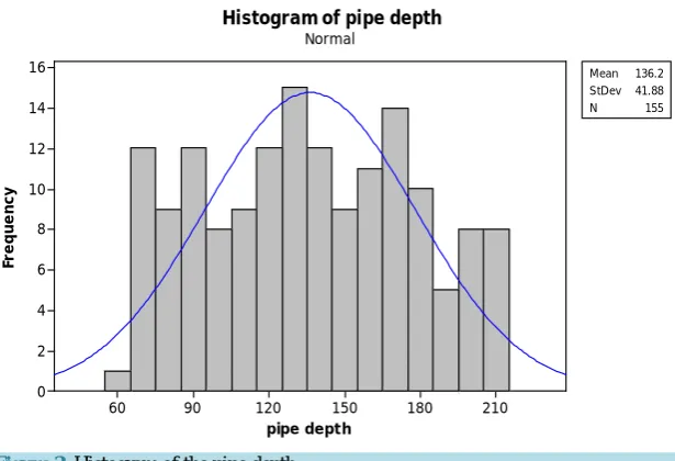
Figure 1displays the histogram for the pipe age. It can be seen that the age roughly follows a normal distribu-tion. Figure 2and Figure3displays the histogram for pipe diameter and pipe installation depth. Such parame-ters are usually determined according to the flow capacity needs and location characteristics. No normal distri-butions are noticed for such two parameters.

Table 2displays the test results when all variables are included. There is a dummy variable involved in the analysis, which is the pipe material, where 1 refers to the concrete pipe, 2 refers to the clay pipe. By checking the P value in this analysis, it can be seen that the pipe diameter is the least significant factor, followed by the pipe material. The pipe installation depth has a P value of 0.294, which is also greater than the significance level 0.05. It means that the hypothesis of β for the depth equals 0 is accepted. Therefore, the depth is not of signifi-cant impact. Both the constant and the pipe age are very signifisignifi-cant to the model.

Figure 1.Histogram of the pipe age.

Table 2. Fitting with all variables included.

Pipe material

1. Pipe index = 0.657119 + 0.0926041 pipe age + 3.66928e−005 pipe diameter + 0.000892305 pipe depth

2. Pipe index = 0.702251 + 0.0926041 pipe age + 3.66928e−005 pipe diameter + 0.000892305 pipe depth

Coefficients

Term Coef SE Coef T P

Constant 0.679685 0.181897 3.7367 0.000

Pipe age 0.092604 0.002947 31.4209 0.000

Pipe diameter 0.000037 0.000954 0.0385 0.969

Pipe material

1 −0.022566 0.035253 −0.6401 0.523

Pipe depth 0.000892 0.000847 1.0538 0.294

Summary of model

S = 0.431973 R-Sq = 86.99% R-Sq(adj) = 86.64%

PRESS = 29.8366 R-Sq(pred) = 86.13%

50 40

30 20

10 0

30

25

20

15

10

5

0

pipe age

Fr

eq

ue

nc

y

Mean 24.55 StDev 11.96

N 155

Histogram of pipe age

Figure 2. Histogram of the pipe diameter.

Figure 3.Histogram of the pipe depth.

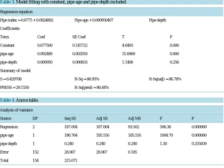
In the following analysis, the constant and pipe age are included in the model. Although the pipe diameter does not seem to be a very significant variable, considering the P value (0.294) is not very great, it is also in-cluded in the model. The new fitting results are shown inTable 3. The results verify that both the constant and the pipe age are governing factors. The pipe depth has a P value of 0.256. It also has an impact on the modeling. Table 4 shows the results for the ANOVA test. Such variance analysis also shows the importance of pipe age and the constant in the model fitting.

Figure 4 illustrates the residual analysis. The normal probability plot shows that most points are clustered around the blue line. It indicates that the error terms are approximately normally distributed. Therefore, the as-sumption of normality is valid. The error terms versus the fitted values figure on the upper right shows that ap-proximately half are above and half are below the zero line. It indicates that the assumption of errors with means of 0 is valid. The histogram is the re-checking of the normality assumption. It fits a normal distribution decently. The figure on the lower right shows that half points are above the line and half points are below the line. It means that the error terms are independent on the time variable.

Therefore, based on the available data, the model generated is

pipe index=0.678 0.092 pipe age+ × +0.00095 pipe depth× 180

150 120

90 60

30 30

25

20

15

10

5

0

pipe diameter

Fr

eq

ue

nc

y

Mean 107.0 StDev 37.05

N 155

Histogram of pipe diameter

Normal

210 180

150 120

90 60

16

14

12

10

8

6

4

2

0

pipe depth

Fr

eq

ue

nc

y

Mean 136.2 StDev 41.88

N 155

Histogram of pipe depth

Figure 4.Residual information for the model fitting.

Table 3.Model fitting with constant, pipe age and pipe depth included.

Regression equation

Pipe index = 0.6775 + 0.0924892 Pipe age + 0.000950407 Pipe depth

Coefficients

Term Coef SE Coef T P

Constant 0.677500 0.145722 4.6493 0.000

pipe age 0.092489 0.002918 31.6969 0.000

pipe depth 0.000950 0.000833 1.1406 0.256

Summary of model

S = 0.429708 R-Sq = 86.95% R-Sq(adj) = 86.78%

PRESS = 29.1550 R-Sq(pred) = 86.44%

Table 4. Anova table.

Analysis of variance

Source DF Seq SS Adj SS Adj MS F P

Regression 2 187.004 187.004 93.502 506.38 0.000000

pipe age 1 186.764 185.516 185.516 1004.70 0.000000

pipe depth 1 0.240 0.240 0.240 1.30 0.255839

Error 152 28.067 28.067 0.185

Total 154 215.071

1.0 0.5 0.0 -0.5 -1.0 99.9 99 90 50 10 1 0.1 Residual P er ce nt 6 4 2 1.0 0.5 0.0 -0.5 -1.0 Fitted Value R es id ua l 0.9 0.6 0.3 0.0 -0.3 -0.6 16 12 8 4 0 Residual Fr eq ue nc y 150 140 130 120 110 100 90 80 70 60 50 40 30 20 10 1 1.0 0.5 0.0 -0.5 -1.0 Observation Order R es id ua l

Normal Probability Plot Versus Fits

Histogram Versus Order

4. Conclusion

This paper develops a model to predict the condition of sewer mains. Based on the available data, it shows that among all available variables, the pipe age is the most significant factor. The pipe installation depth also has an impact in the regression analysis. The pipe material and pipe diameter are found to be less important. The re-gression generates a very decent model, with R square of 0.87 obtained. The ANOVA analysis re-emphasizes the importance of the pipe age variable. The residual analysis shows that the normality assumption of applying the linear model is valid. Although sewer mains are impacted by various factors which also differ significantly from municipality to municipality. The derived equation may not be directly used in other sewer systems. How-ever, the method used and developed can be applied in the analysis of other sewer mains condition when rele-vant data are available.

References

[1] Chughtai, F. and Zayed, T. (2007) Sewer Pipeline Operational Condition Prediction Using Multiple Regression. Pro-ceedings of Pipelines 2007: Advances and Experiences with Trenchless Pipeline Projects.

[2] Moselhi, O. and Shehab-Eldeen, T. (2000) Classification of Defects in Sewer Pipes Using Neural Networks. Journal of Infrastructure Systems, 6, 97-104. http://dx.doi.org/10.1061/(ASCE)1076-0342(2000)6:3(97)

[3] Ariaratnam, S.T., El-Assaly, A. and Yang, Y. (2001) Assessment of Infrastructure Inspection Needs Using Logistic Models. Journal of Infrastructure Systems, 7, 160-165. http://dx.doi.org/10.1061/(ASCE)1076-0342(2001)7:4(160) [4] Jin, Y. and Mukherjee, A. (2014) Markov Chain Applications in Modelling Facility Condition Deterioration.

Interna-tional Journal of Critical Infrastructures, 10, 93-112. http://dx.doi.org/10.1504/IJCIS.2014.062965

[5] Jin, Y. and Mukherjee, A. (2012) Analysis of Heterogeneity in Infrastructure Condition Assessment Models. Construc-tion Research Congress 2012: Construction Challenges in a Flat World, 2241-2249.

http://dx.doi.org/10.1061/9780784412329.225

[6] Jin, Y. (2013) Evaluating Infrastructure Performance to Assist Facility Management toward Sustainable Systems. http://digitalcommons.mtu.edu/etd-restricted/104/

[7] Morcous, G. (2006) Performance Prediction of Bridge Deck Systems Using Markov Chains. Journal of performance of Constructed Facilities, 20, 146-155. http://dx.doi.org/10.1061/(ASCE)0887-3828(2006)20:2(146)

[8] Micevski, T., Kuczera, G. and Coombes, P. (2002) Markov Model for Storm Water Pipe Deterioration. Journal of In-frastructure Systems, 8, 49-56. http://dx.doi.org/10.1061/(ASCE)1076-0342(2002)8:2(49)

[9] Madanat, S.M., Karlaftis, M.G. and McCarthy, P.S. (1997) Probabilistic Infrastructure Deterioration Models with Pan-el Data. Journal of Infrastructure Systems, 3, 4-9. http://dx.doi.org/10.1061/(ASCE)1076-0342(1997)3:1(4)

[10] Yang, J., Gunaratne, M., Lu, J.J. and Dietrich, B. (2005) Use of Recurrent Markov Chains for Modeling the Crack Performance of Flexible Pavements. Journal of Transportation Engineering, 131, 861-872.

http://dx.doi.org/10.1061/(ASCE)0733-947X(2005)131:11(861)

[11] Rowe, R., Kathula, V. and Kelly, B. (2004) Combining Sewer Failure Consequences with Condition Assessment Like-lihood Produces Realistic Prioritization Ranking. Proceedings of the Water Environment Federation, No. 16, 876-889. http://dx.doi.org/10.2175/193864704784147368

[12] Jin, Y. and Mukherjee, A. (2010) Modeling Blockage Failures in Sewer Systems to Support Maintenance Decision Making. Journal of performance of Constructed Facilities, 24, 622-633.

http://dx.doi.org/10.1061/(ASCE)CF.1943-5509.0000126

[13] Jin, Y. and Mukherjee, A. (2010) Analyzing Municipal Blockage Failure Datasets for Sewer Systems. Construction Research Congress 2010: Innovation for Reshaping Construction Practice, 597-606.

http://dx.doi.org/10.1061/41109(373)60

[14] Mukherjee, A., Johnson, D., Jin, Y. and Kieckhafer, R. (2009) Using Situational Simulations to Support Decision Making in Co-Dependent Infrastructure Systems. International Journal of Critical Infrastructures, 6, 52-72.

http://dx.doi.org/10.1504/IJCIS.2010.029576