http://dx.doi.org
Spa
ABSTRAC
This paper pro in the case of basis and the pervised offlin an incrementa need the numb location estim
Keywords: D Pr
1. Introduc
Wireless loca fields like com radio astronom past decade. T zation problem signal parame time of arrival dinates of unk ploiting the p though most l centrate on th eral as explai novel DPD m indeed interes have been pr nique that is s step methods criterion gathe single emitter proach to trea measurement-DPD method g/10.4236/cn.20
arsity-B
1 The Na 2 The Jiangsu 3 Key LCT
oposes an adap f time-varying
sparse solutio ne DL by usin al fashion to ad ber of emitters mation accuracy
Dictionary Lear rogramming
ction
alization as a mmunications, my has drawn The traditional m consists of t eters such as l (TOA) are es known-location parameters est
ocalization alg he two-step me ined in referen methods that di st to the end-u roposed, as a shown to outp
[2]. Weiss et
ering all signa r [3] and then at the multiple
to-association can provide su
013.53B2077 Pu
Based D
Two-st
Ting
Jiangsu Engine anjing Universit u Key Laboratory
N Laboratory of Di
aptive sparsity-channels. The on based on a ng the quadrati
dapt to the tim s aprior. Sim y.
rning; Compre
fundamental radar, sonar, n increasing a l approach to s two-step proce angle of arriv stimated, and s n targets are ca timated in the gorithms presen ethod, it is sub
nces [1]. Rece irectly estimat user, i.e., positi promising po perform the con
t al proposed als of all statio
n proposed a e emitters case step is avoided uperior localiz
ublished Online
Direct L
tep Dic
gting Wang1,2
eering Center of ty of Informatio y on Optoelectr Nanjing Norm U
isaster Reductio Ministry of Civ Email: w
Recei
-based direct p e novel feature two-step dicti ic programmin me-varying cha mulation results
essive Sensing;
task in variou seismology an attention in th solve the local edure. First, th val (AOA) an second the coo alculated by ex e first step. A
nted so far con boptimal in gen ently, a kind o te the results o ion coordinate ositioning tech
nventional two a unique DP ons firstly for
decoupled ap e [4]. Since th d, the decouple zation capabilit
September 2013
ocation
ctionary
2,3, Wei Ke2,3
f Meteorological n Science and T onic Technolog University, Nanj on and Emergen vil Affairs, Beijin wkykw @sina.co
ived May 2013
position determ e of this metho onary learning ng approach, a annel during th s demonstrate
; Direct Locati
us nd he li-he nd or- x- Al- n-of of es, h-o- D a p-he ed ty in mult initial p to be kn method [5,6]. B of supp function higher exploit Com of atten in the t mensio are few rate DP Picard a sity rep fitting m mise th tionary In prac channe mismat mation 3 (http://www.sc
n Estima
y Learn
3, Gang Liu2
l Sensor Networ Technology, Nan
y, School of Phy ing, China cy Response En ng, China om
mination (DPD od is to dynam g (DL) framew and then the d he online stage
the performan
ion; Time-Vary
ti-emitter conte position estima
nown apriori. d to handle th Basically, the a
port points in w n is evaluated. complexity tha the explicit ge mpressed sensin ntion in recent two-step local ons of measure w works discus PD estimation.
and Weiss trea presentation b method in [9]. hat the predefi ) is ideal and i ctice, due to t ls and random tch the actual s
performance cirp.org/journal/
ation B
ning
rk Technology, njing, Chinaysics and Techn
ngineering of the
D) appoach to mically adjust b work. The met dictionary is co
e. Furthermore nce of the prop
ying Channel;
ext. But this m ates, and the nu
Other studies h e global navig above DPD alg which the max Therefore, the an the two-step eometric relati ng (CS), which
years, has bee lization metho ement vectors ssing the CS p To the best o at the DPD pro by exploiting However, thi ined overcomp invariable in th the dynamical m noise, the signals stochas is degraded. I
/cn)
Based on
nology,
e
locate multipl both the overc thod first perfo ontinuously up e, the method posed algorithm
Quadratic
method depend umber of sourc have extended gation satellite gorithms gener ximum likelih ese DPD metho
p approach, w onship. h receives a gr en successfully od by reducing [7,8]. Howev pattern for mo of our knowled oblem as a spat the covarianc s work makes plete basis (a. he localization l change of m
predefined ba stically so that In this paper,
n
e targets complete orms su-pdated in does not m on theds on the ces needs the DPD e system rate a set
ood cost ods have which can
pro-pose an adaptive sparsity-based DPD (ASDPD) algorithm to dynamically adjust both the overcomplete basis and the sparse solution so that the solution can better match the actual scenario. The method first performs supervised of-fline dictionary training by using the quadratic program-ming approach. During the online stage, the dictionary is continuously updated in an incremental fashion to adapt to time-varying factors.
The notation used in this paper is according to the convention. Symbols for matrices (upper case) and vec-tors (lower case) are in boldface. ( )⋅H, θ0, θ1, θ2,
N
I , ⊗ and CN denote conjugate transpose (Hermitian),
0
l norm, l1 norm, l2 norm, identity matrix with the
dimension N, the Kronecker product and complex Gaus-sian distribution, respectively. For any matrix Y, vec( )Y
is denotedasthe vertical concatenation of the columns of
Y. Finally, xˆ denotes the estimate of the parameter of interest x.
The remainder of the paper is organized as follows. Section 2 briefly describes the system model assumed throughout this paper and formulates as a sparse recovery problem. In Section 3, we introduce a scheme calibrating the overcomplete basis dynamically and estimating the sparse solution adaptively. Simulation results are given in Section 4. Finally, Section 5 concludes the paper.
2. System Model and Problem Formulation
Consider N base stations (BS) intercepting the narrow-band signals transmitted by L possible sources. Each BS which knows its coordinates is equipped with an antenna array consisting of M elements. Denote the lth unknown target position by the vector of coordinates Pl. We use
the far-field point-target model, which is commonly used for source localization due to its simplicity [3,4,9]. Based on this model, the received signal observed by the nth BS is given by
1
( ) ( ) ( ( )) ( ) , 0 L
n n l l n l n
l
t s t τ t t T
=
=
− + ≤ ≤r a p p v (1)
where s tl( ) is the signal waveform considered known.
( ) n l
a p is the array response at the nth BS from a signal transmitted position, and the propagation delay from the
lth transmitter to the nth BS is given by τn(pl). The vector
r
n=
H
nθ
+
v
n,
n
∈
{1,
, }
N
represents noise terms, which is assumed as the independent and identi-cally distributed (i.i.d.) complex Gaussian process, un-correlated with the signals.We divide the area of interest into K grids. In general,
KM >L. Then, we formulate the location problem as a following CS problem
, {1, , } n= n + n n∈ N
r H θ v (2)
where ( ) ( ) 1
[ n , , n ]
n = K
H h h is an overcomplete basis ma-trix at the nth BS, and ( )n
i
h corresponds to the noiseless
signal vector between the ith grid and the nth BS.
1
[ ,θ ,θK]
=
θ is a sparse vector that having in total L
nonzero entries, where the indices of nonzero entries in
θ which represents the actual locations. It should be emphasized that the above matrix Hn is constructed by
ideal signals, where the parameters such as AOA and TOA can be calculated according to the geometric rela-tionship directly. Denote H the matrix obtained by concatenation of all the matricesHn, i.e.,
1
[ T, , T]T N
=
H H H . Similarly, by denoting
1
[ T, , T T] N
=
R r r and [ 1, , ]
T T T N
=
V v v , we can obtain
= +
R Hθ V (3)
Note that H is known under the ideal channel condi-tion, which means that we can estimate the actual coor-dinates of targets as long as we find the positions of nonzero values in θ. That is, the problem of localization is converted into one of sparse signal recovery from (3). Moreover, the number of these dominant nonzero values gives L.
However, the non-ideal factors are inevitable in a prac-tical localization system. These factors include the chan-nel attenuation, phase error, time-varying fluctuations of the radio channel and so forth. When these happen, the predefined dictionary cannot effectively express the ac-tual signal, which will cause performance degradation in sparse recovery process.
For avoiding the difficulty of estimate all kinds of the time-varying factors, we assume the error dictionary ma-trix Γ which describe the difference between the prede-fined dictionary and the practical received signals. Note that the error matrix Γ is time-varying and cannot be known in advance. In this scenario, the sparse position-ing model is correspondposition-ingly modified as:
= + +
R ΓHθ V D θ V (4)
where D=ΓH denotes the actual overcomplete basis with the time-varying interference. To prevent D from having arbitrarily large values (which would lead to arbi-trarily small values of θ), it is common to constrain its columns d1,,dK to have a l2 norm less than or
equal to one. Obviously, the mismatch exists between the columnsof D and the corresponding columns of the pre-defined basis H, and thus the performance degradation is inevitable in the sparse recovery process. Focused on this problem, an adaptive sparse recovery algorithm is proposed in this paper, which dynamically calibrate the overcomplete basis so that the sparse solution can better fit the actual scenario.
3. Sparse Representation Based on the
Two-stage Dictionary Learning
tive adjustment of the overcomplete basis. This process generally learns the uncertainty of the dictionary, which is not available from the prior knowledge, but rather has to be estimated using a given set of training samples. Several different DL algorithms have been presented re-cently [10]. However, these methods generally cannot effectively handle very large training sets or dynamic training data changing over time. To overcome these shortcomings, we propose a two-stage DL approach that can adapt to the varied upcoming samples.
So far, the most DL methods are generally based on alternating minimization. In one step, a sparse recovery algorithm finds sparse representations of the training sam-ples with a fixed dictionary. In the other step, the dictio-nary is updated to decrease the average approximation error while the sparse coefficients remain fixed. The pro-posed method in this paper also uses this formulation of alternating minimization.
3.1. Sparse Recovery Phase
The above problem of noisy sparse signal recovery can then be converted into a following optimization problem
2
2 1
min R D− θ / 2+λ θ (5)
where λ is the regularization parameter. However, it should be emphasized that larger coefficients in θ are penalized more heavily in the l1 norm than smaller
coef-ficients, unlike the more democratic penalization of the
0
l norm [11]. In practice, large coefficients are usually the entries corresponding to the actual positions of tar-gets, while small coefficients commonly represent the noise entries. The imbalance of the l1 norm penalty will
seriously influence the recovery accuracy, which may result in many false targets. Therefore, in this paper we choose the reweighted l1 norm minimization algorithm
in [11] as our sparse recovery method, which can over-come the mismatch between l0 norm minimization and
1
l norm minimization while keeping the problem solva-ble with convex estimation tools.
3.2. Dictionary Learning Phase
In this paper, we propose a two-stage DL framework in which the offline DL method allows to train the dictio-nary in a supervised manner to integrate the large train-ing sets, and the incremental DL method based on the results in the offline stage handles the unseen online var-iation to enhance its adaptability.
1) Offline dictionary learning
In this stage, the ideal overcomplete basis H is op-timized to better represent the data of the training sets. Since the sparse coefficients θ are fixed in the DL stage, the resulting optimization problem becomes:
2 2
min R D− θ / 2, s t. .d dHi i≤1,i=1,,K (6)
in which R D− θ22can be written as
2
2 tr[( ) ( )]
tr( ) 2tr( ) tr( ) vec( ) ( )vec( )
2vec( ) vec( ) tr( ) H
H H H H H
H H H H
H H H H
− = − −
= − +
= ⊗
− +
R Dθ R Dθ R Dθ
Dθθ D Rθ D RR
D I θθ D
θR D RR
(7)
Let’s introduce several new expressions for clarity of notation
vec( )
vec( )
H
H
H
⊗
α D
G I θθ
γ θR
Omitting the terms that do not depend on D, the objec-tive function in (6) can be equivalent to
1
min , . . 1, 1, , 2
H H H
i i
s t i K
− ≤ =
α Gα γ α d d (8)
Note that (8) is a standard form of constrained qua-dratic programming problem which can be solved by any standard optimization method, such as the gradient pro-jection algorithm in [12]. Moreover, the matrix G is ob-viously a positively definite matrix, and thus (8) is con-vex function and can be guaranteed to find a global op-timum [13] in this DL phase.
2) Online dictionary learning
Although the offline DL stage has adjust the overcom-plete basis according the training data, it is impossible to be fit for all kinds of time-varying interference patterns. Moreover, its computation load is quite large for real- time localization. On the contrary, the online incremental learning is especially applicable when one seeks to find the variation in the sense that the time-varying channels pattern might not be specifically learned offline but can be distinguished from the past online observations. Based on the incremental learning pattern, the online learning algorithm in [14] can use the result of the offline DL stage as a warm restart for computing the next dictionary where the new samples will be fed into the online dictio-nary learning procedure, and thus a single iteration has empirically been found to be enough [14].
For completeness, a full description of the algorithm is given in Algorithm 1.
Algorithm 1 Two-stage DL algorithm
Initialization: set the training sample set; generate the ideal dictionary
H
Offline DL stage:
Input: the training sample set; (0) off
ˆ =
D H; the number of itera-tions T;
for j=1 to T
( j) off
ˆ
θ with ( 1) off
ˆ j−
D fixed for each sample;
2) use the gradient projection algorithm to minimize the objec-tive function in (8) with respect to ( )
off
ˆ j
D keeping ( j) off
ˆ
θ
fixed; end for
Output: (T )
off off
ˆ =ˆ
D D ; (T )
off off
ˆ =ˆ
θ θ ;
Online DL stage:
Input: (0) on off
ˆ =ˆ
D D ; (0)
on off
ˆ =ˆ
θ θ ; the latest observation samples; 1) update the pre-trained dictionary according to the latest observations using the online DL algorithm in [14] with Dˆoff
as warm restart, and return the learned dictionary (1) on
ˆ
D ; 2) use the reweighted 1-norm algorithm to minimize the
objec-tive function in (6) with respect to (1) on
ˆ
θ keeping (1) on
ˆ
D fixed;
3) (0) (1) on on
ˆ =ˆ
D D ; ( 0) (1)
on on
ˆ =ˆ
θ θ ;
Output: (1)
on on
ˆ =ˆ
D D ; (1)
on on
ˆ =ˆ
θ θ ;
4. Simulation Results
In order to examine the performance of the proposed ASDPD method, we compare it with the decoupled DPD approach in [4] and covariance-based sparse DPD (CDPD) method [9]. Consider four BSs placed at the corners of a 1 km × 1 km square. Assume the number of grids in the location area is K =26 26× , which means yielding a 40m resolution along both x and y axes. The carrier fre-quency of the simulated signal is assumed to be 900 MHz. Each BS is equipped with a uniform linear array of ten antenna elements with the adjacent elements spacing of half a wavelength. The locations of targets are selected at random, uniformly, within the square. All the simula-tion results are obtained based on 200 Monte Carlo rea-lizations. In each simulation, we consider the following multipath channel model
1
( ) ( )
Q
i i
i
cτ β δ τ τ
=
=
− (9)to obtain a set of channel data. { }βi is a et of indepen-dent and iindepen-dentically distributed (i.i.d.) random variables which satisfy (0, bi)
i CN e
τ
β − . b = 1/16 is the
expo-nential power delay profile and τi is the delay spread
for the ith path [15].
[image:4.595.56.291.72.276.2] [image:4.595.315.534.276.473.2]As shown in Figure 1, the improvement in location accuracy for the proposed method can be seen in terms of the root mean square error (RMSE), when the number of emitters is two and the SNR is set to 5 dB. We can ob-serve that the location performance of DPD and CDPD algorithms decreases evidently as the number of multi-path increases. On the contrary, the variation of RMSE in the ASDPD algorithm is very small due to its adaptive ability through DL technique. This result reveals that our method is very robust to multipath channels and effec-tively enhances location accuracy.
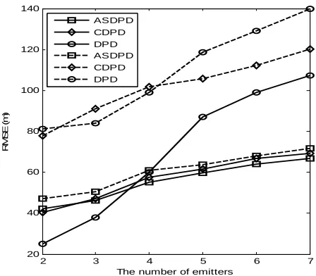
Figure 2 illustrates the location error with respect to
[image:4.595.313.537.513.709.2]the number of emitters when the SNR is set to 5 dB. Here, real lines describe the case of single-path channel for three algorithms, while dashed lines represent the case of three paths. With the increase in the number of emitters, the RMSE of DPD algorithm increases quickly due to the high sensitivity to the estimated number of targets. Note that the CDPD method does not rely on a good estimate of the number of emitters in the single-case, but its per-formance decreases evidently as the number of multipath increases. On the contrary, the ASDPD algorithm is very robust to two scenarios. The importance of the low sensi-tivity of our algorithm to the number of targets is twofold: first, the number of sources is usually unknown, and second low sensitivity provides robustness against mistakes in estimating the number of targets.
Figure 1. The localization error with respect to the number of multipaths.
Figure 2. The localization error with respect to the number of emitters.
1 2 3 4 5
20 40 60 80 100 120 140
The number of multipahs
RM
S
E
(
m
)
ASDPD CDPD DPD
2 3 4 5 6 7
20 40 60 80 100 120 140
The number of emitters
R
M
SE (
m
)
5. Conclusion
In this paper, we exploit the inherent spatial sparsity to present a novel direct location method by combining the offline training and online learning into a unified DL framework, thereby better matching time-varying scena-rios. The effectiveness of the proposed scheme has been demonstrated by simulation results where substantial im-provement for localization performance is achieved. Fur-ther research will emphasize on the off-grid error analy-sis and the theoretic bound on the location estimation precision.
6. Acknowledgements
This work is supported in part by the priority academic program development of Jiangsu higher education insti-tutions, and in part by the Open Research Fund of Key Laboratory of Disaster Reduction and Emergency Response Engineering of the Ministry of Civil Affairs under grant No. LDRERE20120303.
REFERENCES
[1] J. Bosse, A. Ferréol, C. Germond and P. Larzabal, “Pas- sive Geolocalization of Radio Transmitters: Algorithm and Performance in Narrowband Context,” Signal Pro- cessing, Vol. 92, No. 4, 2012, pp. 841-852.
http://dx.doi.org/10.1016/j.sigpro.2011.09.008
[2] A. Amar and A. J. Weiss, “New Asymptotic Results on Two Fundamental Approaches to Mobile Terminal Loca- tion,” Proceedingsof 2008 ISCCSP, pp. 1320-1323. [3] A. J. Weiss, “Direct Position Determination of Narrow-
band Radio Frequency Transmitters,” IEEE Signal Pro- cessingLetters, Vol. 11, No. 5, 2004, pp. 513-516. http://dx.doi.org/10.1109/LSP.2004.826501
[4] A. Amar and A. J. Weiss, “A Decoupled Algorithm for Geolocation of Multiple Emitters,” Signal Processing, Vol. 87, No. 10, 2007, pp. 2348-2359.
http://dx.doi.org/10.1016/j.sigpro.2007.03.008
[5] P. Closas, C. Fernandez-Prades and J. Fernandez-Rubio, “Maximum Likelihood Estimation of Position in GNSS,”
IEEESignalProcessing Letters, Vol. 14, No. 5, 2007, pp. 359-362.http://dx.doi.org/10.1109/LSP.2006.888360 [6] P. Closas, C. Fernandez-Prades and J. Fernandez-Rubio,
“Cramér-Rao Bound Analysis of Position Approaches in GNSS Receivers,” IEEE Transactions on Signal Pro- cessing, Vol. 57, No. 10, 2009, pp. 3775-3786.
http://dx.doi.org/10.1109/TSP.2009.2025083
[7] C. Feng, S. Valaee and Z. Tan, “Multiple Target Locali-zation Using Compressive Sensing,” Proceedingsof 2009
GLOBECOM, pp. 1-6.
[8] B. Zhang, X. Cheng, N. Zhang, Y. Cui, Y. Li and Q. Liang, “Sparse Target Counting and Localization in Sen- sor Networks Based on Compressive Sensing ,” Pro- ceedingsof 2011 IEEEINFOCOM, pp. 2255-2263. [9] J. S. Picard and A.J. Weiss, “Localization of Multiple
Emitters by Spatial Sparsity Methods in the Presence of Fading Channels,” Proceedings of 2010 WPNC, pp. 62-67.
[10] R. Rubinstein, A. M. Bruckstein and M. Elad, “Dictiona- ries for Sparse Representation Modeling,” Proceedings of IEEE, Vol. 98, No. 6, Jun. 2010, pp. 1045-1057.
http://dx.doi.org/10.1109/JPROC.2010.2040551
[11] E. J. Candes, M. B. Wakin and S. P. Boyd, “Enhancing Sparsity by Reweighted l1 Minimization,” Journal of
Fourier Analysis and Applications, Vol. 14, No. 5-6, 2008, pp. 877-905.
http://dx.doi.org/10.1007/s00041-008-9045-x
[12] J. Nocedal and S. J. Wright, “Numerical Optimization,” Springer Verlag, New York, 2006.
[13] J. Dattorro, “Convex Optimization and Euclidean Dis- tance Geometry,” Meboo Publishing, Palo Alto, 2005. [14] J. Mairal, F. Bach, J. Ponce and G. Sapiro, “Online
Learning for Matrix Factorization and Sparse Coding,”
Journal of Machine Learning Research, Vol. 11, No. 3, 2010, pp. 19-60.
[15] M. R. Raghavendra and K. Giridhar, “Improving Channel Estimation in OFDM Systems for Sparse Multipath Channels,” IEEESignalProcessingLetters, Vol. 12, No. 1, 2005, pp. 52-55.