Performance of Bayesian Latent Factor Models in Measuring Pricing Errors

(1)

Munich Personal RePEc Archive

Performance of Bayesian Latent Factor

Models in Measuring Pricing Errors

Chadwick, Meltem

Central Bank of the Republic of Turkey

December 2010

(2)

Performance of Bayesian Latent Factor Models in

Measuring Pricing Errors

∗

Meltem G¨

ulenay Chadwick

†

Abstract

This study offers a Bayesian factor modelling framework to obtain the exact distri-bution of pricing errors in the bounds of Arbitrage Pricing Theory with the aim of observing, first if the usage of a dynamic model, second increasing the number of factors beyond one contributes to a significant reduction of the pricing errors ob-tained. In doing so, we compare the pricing errors we get from a static and dynamic latent factor model, while adopting the Fama-French data for US monthly industry returns. We observe that the pricing errors increase slightly using a dynamic factor model, when compared with the static factor model. Besides, inclusion of factors beyond the first one pose an improvement with respect to the pricing errors both for the static and the dynamic factor model. When we introduce time-varying betas to the dynamic factor model we get the lowest pricing errors at t_{= 1 compared to}

static and dynamic model with fixed betas, where the mean pricing errors decreased by 33 percent compared to the static model. Yet pricing errors also become time varying as their dynamics now depend on the dynamics of beta.

Keywords: arbitrage pricing theory; Bayesian dynamic factor model; pricing errors; Fama-French industry returns

JEL Code: C11, C58, G12

∗_{This article is a part of the PhD dissertation of the author completed under the supervision of Zacharias Psaradakis and}

Stephen Satchell. I am indebted to my PhD supervisors and I thank the participants at the Birkbeck College/University of London doctoral seminar, the Central Bank of Turkey Research and Monetary Policy department seminar, the 5th International Conference on Computational and Financial Econometrics for their valuable comments. I also thank George Kapatenios, T¨uralay Ken¸c and Haroon Mumtaz for their assistance. The views expressed herein are those of the author and not necessarily those of the Central Bank of Turkey. Any remaining mistakes are my own.

(3)

1 Introduction

Factor models have been very popular in finance with applications in the area of Arbitrage Pricing Theory (APT) and especially Capital Asset Pricing Model (CAPM) of asset prices. APT implies that expected asset return is a linear function of the risk premium on systematic factors of economy. Starting point of the usage of factor models in applications to APT goes back to King (1966) who shows that there are market and industry factors in security returns. One of the commonly cited rigorous proofs of APT was introduced by Ross(1976) providing an approximate relation for expected asset returns with an unknown number of unidentified factors in a competitive and frictionless market.1 _Until _{Chen et al.} ₍₁₉₈₆_),

empirical applications of APT were based on factor analysis of security returns. Chen et al.

(1986) show how APT may be estimated and applied, using macroeconomic factors.2

While the academic literature on APT is developing on a faster pace, another line of research is concerned with testing whether the models developed using APT can represent the real world of asset pricing. In this respect, Gehr (1975) publishes the first test of APT even before Ross (1976) was published, and afterwards his work has been cited by every study accomplished in the area.3 _{One of the arguments against the APT has been the}

approximate nature of its pricing equation. While Chen and Ingersoll (1983) provide some arguments for an exact pricing relationship,Dybvig(1983) andGrinblatt and Titman(1983) provide bounds on the approximation error, also known as the pricing error. One of the most prominent study on pricing errors is byGeweke and Zhou(1996) who analyze the exact pos-terior distribution for the pricing errors using a Bayesian static factor model. In this respect, this study extends the analysis of Geweke and Zhou (1996) one-step further by obtaining the distribution of pricing errors in a dynamic setup using similar Gibbs Sampling/Data Augmentation methods. In this way, we aim to observe if the pricing errors obtained from a static model will diminish using a model closer to real life asset pricing dynamics. This

1

Chamberlain(1983) andIngersoll(1984) are other significant treatments of APT. For example,Connor(1984) derives an equilibrium (as opposed to no-arbitrage) version of APT.Nawalkha(1997) provides a good synthesis of many issues related to CAPM, multifactor models, and APT.

2

Burmeister and Wall(1986) also use macroeconomic factors to explain APT.

3

(4)

paper will present if there will be improvements of pricing error over a static Bayesian latent factor model, and show that when we include time-varying dynamics to a static model the density of the pricing error also varies over time. Therefore the pricing error measure ala

Geweke and Zhou (1996) looses its significance to use as a comparison unit over different models. Therefore, we only compare static factor model with the dynamic factor model that has fixed betas.

Following the multifactor pricing within APT literature, it can easily be observed that linear static factor models dominate the literature and they are the most widely used tools to value return on risky assets. By introducing a dynamic model, co-movement of different assets will also be incorporated into the analysis. Although the theory maintains a linear and stable relationship between risk factors and returns, it does not postulate a static structure for the factors. This is perhaps not very surprising because the theoretical underpinnings of the unconditional APT reveal that time-invariant linear factor structures are only obtained when one imposes strong assumptions on the underlying probability distributions and investors’ attitudes towards risk. In that respect, if the true data generating process for returns has a dynamic structure, then pricing errors obtained from static factor model will be diminished significantly with reduction of misspecification error, as using a static data generating process for a dynamic procedure will cause pricing errors to increase. However, one should be very cautious about introduction of extra parameters to the model with the usage of dynamic structure, as the introduction of wrong dynamics will cause the estimation error to increase. Yet the shift of focus from static factor models to dynamic factor models resulted from the basic difficulty of examining the empirical support for the static models especially the CAPM, which is related to the fact that the real world is inherently dynamic and not static. Many studies being published in the area of APT raised some doubts about empirical validity of APT.4 _{While tests of APT concerned many academicians, a similar line of debate}

(5)

of the number of factors resulted in development of new modelling techniques and testing procedures given the fact that we can use the pricing errors obtained from models with dif-ferent number of factors as a means to see how well the new model fits into the theory. In this respect we increase the number of factors in each model we estimate, to observe if the pricing errors of estimated models will be affected by using a different factor structure.

Our study contributes to a body of research focusing on different aspects of the asset pricing, financial econometrics and Bayesian modelling literature. The motivation and aim of this paper is closely related to the topic of improving models utilized in APT, making them closer to real asset market dynamics, and examining how many relevant factors explain the pricing equations and minimise the pricing errors. We use Fama and French monthly industry portfolios in the estimation of all of our models as this data set is the most employed set within the APT literature.5 _{We model monthly industry portfolio returns, first with a}

static Bayesian latent factor model, then with a dynamic Bayesian factor model and lastly with a dynamic model where the factor loadings are time-varying. In all of the models used the latent factors and the loading are estimated in one-step. In addition to that, in line with the two studies by Shanken (1992b), and Geweke and Zhou (1996), the measure for pricing errors are adjusted utilizing the approach that has been offered in those two studies, and the distribution for pricing errors is analyzed accordingly.

The rest of this paper is organized as follows. Section 2 lays out a sample version of the Fama and French monthly industry portfolios data set used and gives brief descriptive statistics. In Section 3, we introduce static Bayesian factor model and we explain estimation, identification and pricing errors we get from it. In Section 4, we extend the static factor model introduced in the previous section, estimate and identify a dynamic factor model and get a new set pricing errors. In section 5, we introduce time varying betas to the dynamic factor model and get pricing errors that change over time. Section 6 concludes.

5

(6)

2 Data and Descriptive Statistics

Fama and French (1997) find that the risk loadings of the industry sorted portfolios exhibit great time variation and are difficult to be estimated precisely. To solve this problem, economists added new factors to the three factor model of Fama and French and worked out if the additional factor can solve the problem of variation. Despite the continuing controversy about the interpretation of Fama and French results, their three factor model remains a cornerstone in the literature on cross-sectional asset pricing tests. Yet, there is no model that performs better in explaining the cross-section of average returns on size and book to market sorted portfolios. Since their model is the most referred in the asset pricing literature, we use Fama and French industry portfolio data set as a benchmark. Usage of this specific data set will simplify comparing our results to the results of similar works published within the framework of APT literature.

While estimating the latent factor models and extracting the distribution for the pricing errors we use three groups of industry portfolios. All three groups are the returns on the value weighted industry portfolios grouped by Fama and French.6

In all our estimations we used three groups of industries of which the first group is composed of five, second group is composed of ten and finally third group of data is composed of seventeen industries.7 _{By increasing the number of cross sections, we will be able to}

observe how the pricing errors behave accordingly. Portfolio returns are monthly returns from January 1990 to May 2005; as a result the times series dimension of data set is 185.

6

The empirical results obtained from all of the models utilized in the paper yielded qualitatively and quantitatively very similar posterior distributions for pricing errors when equal weighted portfolios are used as data set, so we do not illustrate the results related to equal weighted industry portfolio data set.

7

(7)

[image:7.612.74.565.94.585.2]

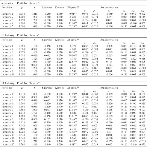
Table 1: Descriptive Statistics of Industry Portfolio Returns

5 Industry Portfolio Returns*

Portfolios µ σ Skewness Kurtosis JB-prob.** Autocorrelation

ρ1 ρ2 ρ3 ρ4 ρ12 ρ24 Industry 1 0.950 1.210 -0.280 3.980 9.91** 0.073 -0.035 -0.089 -0.123 0.077 0.092 Industry 2 1.000 1.200 -0.310 3.540 5.280 -0.045 -0.010 -0.051 -0.064 0.084 0.118 Industry 3 1.120 1.260 -0.030 3.170 0.250 -0.034 0.044 0.013 -0.064 0.054 -0.003 Industry 4 0.980 1.720 -0.390 3.920 11.20** 0.014 -0.012 0.081 -0.081 -0.026 0.057 Industry 5 1.090 1.640 -0.510 4.820 33.35** 0.040 -0.012 -0.066 -0.136 0.007 0.009

ρ1 ρ2 ρ3 ρ4 ρ12 ρ24 Industry 1 0.990 1.130 -0.150 3.780 5.470 0.053 -0.020 -0.139 -0.088 0.119 0.146 Industry 2 0.830 0.980 -0.300 3.470 4.380 0.083 -0.069 0.006 -0.094 0.072 0.003 Industry 3 1.070 1.400 -0.470 3.670 10.14** -0.016 -0.021 -0.085 -0.113 0.081 0.097 Industry 4 1.080 0.630 0.600 4.070 20.00** -0.095 -0.051 -0.065 -0.037 0.069 0.106 Industry 5 1.280 1.420 -0.290 3.500 4.450 0.002 -0.002 0.042 -0.090 -0.022 0.048 Industry 6 0.560 1.080 -0.060 4.290 12.87** 0.042 -0.010 0.113 -0.084 0.004 0.098 Industry 7 1.020 0.890 -0.170 3.260 1.380 0.084 -0.049 -0.044 -0.110 0.068 0.039 Industry 8 1.120 1.260 -0.030 3.170 0.250 -0.034 0.044 0.013 -0.064 0.054 -0.003 Industry 9 0.840 1.130 -0.320 3.420 4.530 0.045 -0.072 0.091 0.031 0.012 0.089 Industry 10 1.090 1.640 -0.510 4.820 33.35** 0.040 -0.012 -0.066 -0.136 0.007 0.009

ρ1 ρ2 ρ3 ρ4 ρ12 ρ24 Industry 1 1.010 1.080 -0.090 4.200 11.39** 0.044 -0.038 -0.152 -0.091 0.138 0.133 Industry 2 0.860 0.900 0.070 3.380 1.290 -0.026 -0.046 -0.002 -0.126 0.051 0.027 Industry 3 1.050 0.620 0.600 3.970 18.46** -0.101 -0.034 -0.058 -0.015 0.062 0.087 Industry 4 0.790 1.270 -0.320 4.420 18.66** 0.206 -0.058 -0.129 -0.134 0.105 0.029 Industry 5 0.680 0.930 -0.490 3.700 11.08** -0.001 0.017 -0.020 -0.145 0.162 0.133 Industry 6 0.860 1.060 0.210 4.120 11.04** -0.042 -0.043 -0.066 -0.110 0.068 0.127 Industry 7 1.140 1.770 -0.160 2.940 0.830 -0.036 0.030 -0.017 -0.101 0.095 0.014 Industry 8 1.190 1.220 -0.150 4.190 11.61** 0.053 -0.085 -0.002 -0.114 0.136 0.087 Industry 9 0.790 0.560 0.120 5.070 33.45** -0.018 -0.020 -0.004 -0.069 0.009 0.009 Industry 10 0.920 1.010 -0.420 4.300 18.49** 0.107 -0.035 -0.080 -0.080 0.046 0.075 Industry 11 1.240 1.050 -0.490 4.230 19.18** 0.005 0.005 0.064 -0.077 0.026 0.059 Industry 12 0.890 1.110 -0.200 3.340 2.180 0.067 -0.087 0.023 -0.071 0.055 -0.032 Industry 13 1.020 1.620 -0.650 4.630 33.58** 0.072 -0.006 -0.031 -0.103 0.008 0.094 Industry 14 0.840 1.130 -0.320 3.420 4.530 0.045 -0.072 0.091 0.031 0.012 0.089 Industry 15 1.040 1.020 -0.100 3.180 0.550 0.088 -0.045 -0.060 -0.084 0.080 0.059 Industry 16 1.310 1.770 -0.340 4.740 26.84** 0.016 -0.001 -0.053 -0.108 -0.003 -0.015 Industry 17 0.760 1.440 -0.440 3.560 8.38** 0.055 -0.049 0.045 -0.110 -0.049 0.073

*Industry definitions are given in Appendix A.

(8)

[image:8.612.180.429.97.558.2]

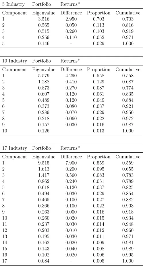
Table 2: Principal Component Analysis

Component Eigenvalue Difference Proportion Cumulative 1 3.516 2.950 0.703 0.703 2 0.565 0.050 0.113 0.816 3 0.515 0.260 0.103 0.919 4 0.259 0.110 0.052 0.971

5 0.146 – 0.029 1.000

Component Eigenvalue Difference Proportion Cumulative 1 5.579 4.290 0.558 0.558 2 1.288 0.410 0.129 0.687 3 0.873 0.270 0.087 0.774 4 0.607 0.120 0.061 0.835 5 0.489 0.120 0.049 0.884 6 0.373 0.080 0.037 0.921 7 0.289 0.070 0.029 0.950 8 0.218 0.060 0.022 0.972 9 0.157 0.030 0.016 0.987

10 0.126 – 0.013 1.000

Component Eigenvalue Difference Proportion Cumulative 1 9.515 7.900 0.559 0.559 2 1.613 0.200 0.095 0.655 3 1.417 0.560 0.083 0.783 4 0.862 0.240 0.051 0.789 5 0.618 0.120 0.037 0.825 6 0.494 0.030 0.029 0.854 7 0.465 0.100 0.027 0.882 8 0.366 0.100 0.022 0.903 9 0.263 0.000 0.016 0.918 10 0.260 0.020 0.015 0.934 11 0.237 0.030 0.014 0.948 12 0.203 0.010 0.012 0.960 13 0.195 0.030 0.011 0.971 14 0.162 0.020 0.009 0.981 15 0.143 0.040 0.008 0.989 16 0.102 0.020 0.006 0.995

17 0.084 – 0.005 1.000

(9)

the ten industry portfolio ranges from 0.56 percent per month to 1.28 percent per month. The lowest standard deviation is found to be 0.63. Considering the mean for seventeen industry portfolio, the mean for the portfolios range from 0.68 percent and 1.31 percent. Last columns of Table (1) give us the autocorrelation coefficients of the industry portfolio data set. A close examination of the coefficients betweenρ1 toρ24 signals an autocorrelation

structure for the data set used.

Table (2) lays out the principal component analysis of the Fama-French industry portfo-lios used for the analysis in the coming sections of the paper. For the five industry portfolio, the difference between the largest eigenvalue 3.52, and the second one 0.56, is substantially large. In addition to that, the first eigenvalue explains 70 percent of the total variation of returns. Principal component analysis points out that for the five industry portfolio returns the first component explains significant amount of the total variation. If we examine ten in-dustry and seventeen inin-dustry portfolio results, the first component explains the biggest total variation and the difference between the first and the second eigenvalue decreases sharply.8

3 Static Model and Pricing Errors

Let us introduce the general form of the static factor model.9 _{In its most commonly used}

form, APT provides an approximate relation for expected asset returns with an unknown number of unidentified factors. One of the important assumptions behind APT is that the markets are competitive and frictionless. In the purest sense, the return generating process

8

Harding(2008) explains the bias of APT models estimated by PCA towards a single factor model.

9

(10)

for asset returns being considered for the system of N assets is:

rt = α+βft+εt (1)

E[ft] = 0

E[ftft′] = I

E[εt|ft] = 0

E[εtε′t|ft] = Σ

In the system equation rt is an (N ×1) vector of returns, α is an (N ×1) vector with

α= [α1 α2 ... αN]′,β is an (N×K)matrix with β = [β1 β2 ... βN]′,ft is an (K×1)

vector andεtis an (N×1) random vector with εt = [ε1 ε2 ... εN]′. It is further assumed

that the factors account for the common variation in asset returns so that the disturbance term for large well-diversified portfolio vanishes. This requires that the disturbance terms be sufficiently uncorrelated across assets. We also make the standard assumptions that εt

and ft are independent and both follow multivariate normal distributions.

The absence of riskless arbitrage opportunities implies an approximate linear relationship between the expected asset returns and their risk exposures as the number of assets satisfying Equation (1) tends towards infinity:10

αi ≈λ0+βi1λ1+...+βiKλK, i= 1, ..., N, (2)

where λ0 is the intercept of the pricing relationship and λk is the risk premium on the

k-th factor. Equation (2) is the implication of no asymptotic arbitrage, and in contrast with the much stronger assumption of competitive equilibrium, Connor’s (1984) equilibrium

10

(11)

version APT replaces the approximation with an equality.11 _{Considering, the measurement}

of pricing errors, we will use the measure offered by Geweke and Zhou (1996):

Q2 = 1

N

X

i=1

(αi−λ0−βi1λ1−...−βiKλK)2. (3)

Q2 _{given in Equation (}₃_{) is the average of the squared pricing errors across the assets.}

Under the strict assumption of competitive equilibrium, Equation (2) becomes an exact relationship, implying that pricing error (Q) is zero. However, for the asymptotic APT, the pricing error converges to zero as the number of assets approach to infinity. On the other hand, if the competitive equilibrium assumption does not hold, pricing error will not converge to zero as long as the number of assets is finite Shanken (1992a).

Following Geweke and Zhou (1996), conditional onαandβ, the minimised mean squared pricing error can be written as:

Q2 = 1

Nα

′

[IN −β∗(β′∗β∗)−1β′∗]α. (4)

where β∗ _{= (1}

N, β) and 1N is an N ×1 vector of ones.

By utilizing the maximum likelihood techniques, the exact sampling distribution of the pricing error is difficult to determine. However, the exact posterior density is easy to con-struct using Bayesian MCMC methods. Therefore, for both the static and dynamic Bayesian factor modelsα andβ are sampled with each iteration of the Gibbs sampler. Since the

pric-11

Ross(1976) assumes that the market, which consists of infinitely many securities is efficient. This assumption is needed to make sure that the total risk of a portfolio is diversifiable. The approximation (≈) in the APT pricing equation arises in economies with finite number of securities because the total risk (variance) of the arbitrage portfolio is not completely diversifiable in a finite economy. Ross(1976),Dybvig(1983) andGrinblatt and Titman(1983) provide theoretical arguments to show that the average pricing error would empirically be negligibly small. Shanken(1982) argues that even if the average pricing error is small, individual pricing errors may be large. Dybvig and Ross(1985) show that Shanken’s arguments hold under very special conditions, which are not likely to be encountered in real situations.Robin and Shukla(1991) show that the pricing errors for some securities are large. A version of the APT based on competitive equilibrium (Chen and Ingersoll(1983),

(12)

ing error is a function ofα and β, it is trivial to compute and store a Markov Chain for the pricing error for each iteration.12 _{The resulting sample provides the exact posterior density}

of the pricing error. The availability of an exact posterior density for a function of param-eters is a significant advantage of the Bayesian approach. In this framework, we derive the posterior distribution of Q for both static and dynamic factor model and use this measure as an informal metric to determine whether pricing errors are economically significant. We then compare model performance using this informal metric.13

Static factor model and the basic assumptions are simply illustrated with Equation (1) above. Letting Θ be the parameter space that is associated with α, β and Σ, the joint posterior density function of the parameters based on Bayes’ rule will be:

P(α, β,Σ)∝ |Σ|−1/2_f₍_R_|_{α, β,}_Σ)

where, R is the T ×N matrix returns andf(R|α, β,Σ) is the density of the data condi-tional on the parameters. We stated that εt ∼N(0,Σ) andft∼N(0, I). Consequently,

R|Θ∼N(f β′

,|Σ)

f(R|Θ) = [(2π)T N|ββ′

+|Σ|T]−1/2_exp_{−₀_.₅_tr₍_ββ′

+ Σ)−1_R′

R}

and the unconditional variance ofrt is, Ω =ββ′+ Σ

The prior density for the factor scores is given byβi :Nk(βi, Bi

−1

). The prior distribution

12

Convergence statistics are illustrated in Appendix B.

13

(13)

for Σ will be accordingly; we will assign an inverse gamma distributions for the σ2

is, that is

σ_i2 ∼IG(ν0i/2, ν0is20i/2)

The information concerning parameters can be controlled by the magnitude of shape parameter of inverted gamma distribution.

For the static factor model used in this part, we should address a small statement about the identification, i.e. the model is invariant under transformations of the form β∗ ₌ _βP′

and f∗

t =P ft, whereP is any orthogonalK×k matrix. There are different ways to identify

the model by imposing constraints on β. The identification method used in this paper is to constrain β in such a manner that the matrix β is a block lower triangular matrix, assumed to be of full rank, with diagonal elements strictly positive. That is:

β =



      

β11 0 . . . 0

β21 β22 . . . 0

... ... ... ...

βK1 βK2 . . . βKK



      

where βii > 0, i = 1, ..., K. This condition uniquely identifies the loadings and the

associated factors. This type of identification procedure is utilised in Geweke and Zhou

(1996) and Aguilar and West (2000). In this form of identification, the loading matrix has

r =N K−K(k−1)/2 free parameters. WithN non-zeroσi parameters, the resulting factor

form of Ω has N(K + 1)−K(K −1)/2 parameters, compared with the total N(N + 1)/2 in an unconstrained model where K =N. In this respect the constraints provide an upper bound on the number of factors that has to be estimated.14

Expected return pricing errors orα’s are useful characterisation of a model’s performance. Analysing them helps to guard against accepting an uninteresting model: one that prices

14

The constraint isN(N+ 1)/2−N(K+ 1) +K(K−1)/2≥0 provides an upper bound on K. For exampleN= 5 implies

(14)

assets badly, but produces large enough standard errors so as not to be rejected by the certain model comparison criteria. It also helps to guard against the equally dangerous possibility of rejecting a good model: one that produces economically tiny pricing errors, with such smaller standard errors that the model is still statistically rejected.

Pricing errors may occur either because the model is viewed formally as an approxima-tion, as in many linear factor pricing models, or because the empirical counterpart to the theoretical APT factor model is error ridden.15 Pricing errors or closely related expected re-turn errors are commonly used to assess asset pricing models. For instance, in linear factors of returns the principle of no-arbitrage is used to characterise the sense in which security market prices can be approximately represented in terms of the prices of a small number of factors.16

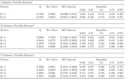
After getting the posterior distribution for both αand β, it is straightforward to find the posterior distribution of a function of them that is Q. The posterior mean of pricing error is provided in Table (3) for static factor model and for all of the industry portfolios used in estimation. The results are reported for the whole sample period, that is from January 1990 to May 2005. The first column of the table refers to the number of factors used when estimating the model.17 _{The second and the third column of Table (}₃_{) report the posterior}

mean and the standard deviation of Q.

15

See Roll’s (1977) critique of the single-period capital asset pricing model.

16

See,Ross(1976),Huberman(1982),Chamberlain and Rothschild(1983) andShanken(1987).

17

(15)

[image:15.612.90.523.96.372.2]

Table 3: Average Pricing Errors with Static Factor Model

Factors Q Std. Error 90% Interval Quantiles

0.025 0.25 0.5 0.75 0.975 K=1 0.1824 0.0805 [0.0499, 0.3147] 0.054 0.124 0.174 0.231 0.363 K=2 0.1647 0.0847 [0.0254, 0.3041] 0.030 0.100 0.155 0.219 0.351

0.025 0.25 0.5 0.75 0.975 K=1 0.2902 0.0793 [0.1598, 0.4207] 0.153 0.232 0.285 0.341 0.463 K=2 0.2644 0.0772 [0.1373, 0.3916] 0.129 0.209 0.258 0.315 0.429 K=3 0.2383 0.0742 [0.1163, 0.3603] 0.108 0.185 0.233 0.286 0.396 K=4 0.2210 0.0693 [0.1069. 0.3350] 0.098 0.172 0.217 0.266 0.369

0.025 0.25 0.5 0.75 0.975 K=1 0.3329 0.0641 [0.2275, 0.4383] 0.222 0.287 0.328 0.373 0.473 K=2 0.3005 0.0619 [0.1987, 0.4023] 0.190 0.258 0.296 0.339 0.435 K=3 0.2607 0.0491 [0.1791, 0.3422] 0.171 0.227 0.258 0.292 0.365 K=4 0.2415 0.0469 [0.1644, 0.3187] 0.154 0.210 0.239 0.272 0.339

(16)

4 Dynamic Model and Pricing Errors

The shift of focus from static factor models to dynamic factor models resulted from the basic difficulty of examining the empirical support for the static models, especially the CAPM, which is related to the fact that the real world is inherently dynamic and not static. There-fore, within this part of the paper we will use the same metric Q to get the density of the pricing errors but in a more complex model where the factors have a lag structure. In the dynamic factor modelling context, the analogue of model that has been represented in Equation (1) can be written as:

rt = α+β(L)ft+εt (5)

ft,K = φ1ft−1,K +...+φqft−q,K +ut, k= 0,1, ..., n

E[ft] = 0

E[ftft′] = I

E[ut|ft] = 0

E[εtε′t|ft] = Σ

Σ = diag(σ₁2, ..., σ_N2 )

where β(L) is an (N ×K) matrix of polynomials in the lag operator, and the errors εt

may be serially, but not necessarily cross sectionally correlated and ut is an i.i.d. innovation,

uncorrelated across factors. We allow the factor loading β(L) to be a lag polynomial to capture the idea that different sectors in the portfolio may respond to the common factors with different lags. In the model, the factors are assumed to evolve as independent AR(q) processes that are invariant over time.

(17)

in the dynamic factor model setup, given as:

εi,t = ψi1εi,t−1+...+ψiqεi,t−q

The notation that will be utilised within the framework of dynamic factor model will be accordingly:

F = [f1, ..., fK]′ Φ =



   

φ11 . . . φ1q

... ... ...

φ1q . . . φqq

     Ψ =     

ψ11 . . . ψ1q

... ... ...

ψ1q . . . ψqq

     β =     

β11 . . . β1K

... ... ...

β1N . . . βN K

     σ2 f =      σ2

1 . . . 0

... ... ... 0 . . . σ2

k      σ2 i =      σ2

1 . . . 0

... ... ... 0 . . . σ2

N     

and α= [α1, ..., αN].

In the model defined above,εtandftare assumed to be independent and follow

multivari-ate normal distributions. In addition, all the innovations of the model are assumed to be zero mean, contemporaneously uncorrelated random variables. Therefore, all the comovement is mediated by the factors, which in turn all have autoregressive representations.

(18)

statistical techniques employing the Kalman filter/smoother to estimate the model parame-ters and extract an estimate of the unobserved factor. However, using the Kalman filter to estimate the model becomes more difficult as the computation of the state equation becomes more and more cumbersome with increasing number of factors. In that respect, an alterna-tive procedure can be based on a recent development in the Bayesian literature on missing data problems, that of “Data Augmentation” proposed by Tanner and Wong (1987). As in static model we use “Data Augmentation” to estimate the dynamic model. In this way, we can compare the pricing errors in a more convenient way.18

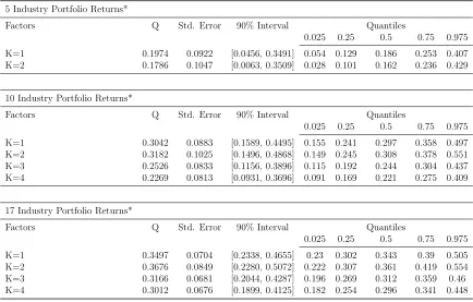
In Table (4) below we illustrate the mean, standard deviation, 90 percent Bayesian in-terval and the quantiles for the pricing errors we get using Bayesian dynamic latent factor model. When we examine the results given in Table (4), we see that the mean for the pricing errors with all three portfolio increases if we compare the results with Table (3). We can argue that in fact both models perform similarly with respect to the examination of the pos-terior distribution of pricing error. Yet, if we want to use the mean pricing errors as a model comparison criteria we can definitely state that the static model outperforms the dynamic model as static model produces smaller pricing errors. More importantly, as in static factor model mean pricing errors decrease as we increase the number of factors. for the 5 industry portfolio this decrease is 9.5 percent. For the 10 and 17 industry portfolios the decrease in the mean pricing errors between the first and fourth factors are 25 percent and 14 percent respectively.

18

(19)

[image:19.612.87.521.96.373.2]

Table 4: Average Pricing Errors with Dynamic Factor Model

0.025 0.25 0.5 0.75 0.975 K=1 0.1974 0.0922 [0.0456, 0.3491] 0.054 0.129 0.186 0.253 0.407 K=2 0.1786 0.1047 [0.0063, 0.3509] 0.028 0.101 0.162 0.236 0.429

0.025 0.25 0.5 0.75 0.975 K=1 0.3042 0.0883 [0.1589, 0.4495] 0.155 0.241 0.297 0.358 0.497 K=2 0.3182 0.1025 [0.1496, 0.4868] 0.149 0.245 0.308 0.378 0.551 K=3 0.2526 0.0833 [0.1156, 0.3896] 0.115 0.192 0.244 0.304 0.437 K=4 0.2269 0.0813 [0.0931, 0.3696] 0.091 0.169 0.221 0.275 0.409

0.025 0.25 0.5 0.75 0.975 K=1 0.3497 0.0704 [0.2338, 0.4655] 0.23 0.302 0.343 0.39 0.505 K=2 0.3676 0.0849 [0.2280, 0.5072] 0.222 0.307 0.361 0.419 0.554 K=3 0.3166 0.0681 [0.2044, 0.4287] 0.196 0.269 0.312 0.359 0.46 K=4 0.3012 0.0676 [0.1899, 0.4125] 0.182 0.254 0.296 0.341 0.448

5 Dynamic Model with Time-Varying Betas and

Pric-ing Errors

In practice, many portfolio managers constantly update and re-estimate factor returns and indeedFerson and Harvey(1991,1993) andFerson and Korajczyk(1995) find that estimated betas exhibit statistically significant time variation.19 _{If we succeed in capturing the}

dynam-ics of beta risk by allowing variation for factor loadings in the dynamic factor model, and if the true data generating process have the time variation for the betas, then it is expected that the model will outperform the previous static model and dynamic factor model where

19

In the majority of the literature, beta is defined to be constant over a certain period of time. However, this static beta result is at contradiction with another line of literature with an early evidence ofBlume(1971) whom finds that beta is time varying.Fama and MacBeth (1973) propose a rolling regression approach to estimate the beta, where they assume that beta is constant only during short time intervals. Fabozzi and Francis(1977) propose a beta that is dependent on the state of the market. Ferson and Harvey (1999) show that the beta is influenced by the macroeconomics variables hence is time varying.

(20)

the betas are fixed. However, if the beta risk is inherently misspecified , there is a real possibility that we commit serious pricing errors that potentially could be bigger than with a constant beta model.

When we allow time varying factor loadings the dynamic factor model that we have described with Equation (1) and (5) will be modified as:

rt = α+βtft+ǫt (6)

Again, the law of motion of the factors is an AR(q) process and ǫt follows an AR(p)

process. The law of motion for the factor loading coefficients follows a random walk without drift, which is the most common usage in the literature. Therefore the dynamics of the beta can be given as:

βt = βt−1+ηt (7)

where, ηt is an i.i.d. disturbance. We assume that all the errors are normally distributed

and uncorrelated with each other. The difference of this model with time varying loadings from the previously estimated dynamic and static factor model is that, the variance of the innovation for the factor is normalized to one. The reason for this normalization is related closely with the identification of the model, i.e. in Equation (6), if we increase the standard deviation offt by a factor of κ and at the same time divide all the βt’s by κ, we will obtain

exactly the same process for the observable. The identification problem is solved in the literature by normalizing the standard deviation of the factor innovation to one and letting the βt’s be unconstrained. A related identification issue is that the sign of the factor and

factor loadings are not separately identified. To solve this problem we follow the conventional approach and normalize the sign of the factor loadings.

(21)

inference from the joint posterior distribution p(F, θ|y). The parameters are represented by

θ. The joint distribution cannot be obtained directly. However, the conditioning features of the model allow us to implement the Gibbs-sampling methodology for Bayesian inference. Gibbs-sampling can be implemented by successive iteration of the following steps given appropriate prior distributions and arbitrary starting values for the model’s parameters. The sampling procedure is very similar to the one described in previous part. We just have extra parameters that come with the introduction of Equation (7).

Q2_t= 1

Nα

′

[IN −β∗t(β

′∗

tβ

∗

t)

−1_β′∗

t]α. (8)

where β∗

t= (1N, βt) and 1N is a vector of ones.

In the third and fourth part of this paper, we used Equation (4) to get the posterior distribution of the pricing errors employing Bayesian static and dynamic factor models. In this part of the paper, we use a GLS type of weighting matrix to adjust the pricing errors given by Equation (8) to see if the weighting matrix will affect the pricing errors. If we will use the mean pricing error as a basis of model comparison, how it is measured gains great importance. Related to the CAPM literature, the minimised errors are defined as Q′_{W Q}_,

where W is the weighting matrix. This method is equivalent to estimating the parameters to minimise the weighted sum of squared pricing errors. When we estimated the static and dynamic factor models in the previous parts we calculated the average pricing errors with weighting matrix that is equal to the identity matrix advocated by Cochrane (1996). The identity weighting matrix gives equal weight to all the moment conditions and examines the ability to price the assets used in the tests. An advantage using the identity weighting matrix is that we can compare the performance across models.20 _{The only assumption needed is}

that the weighting matrix is nonsingular.

20

(22)

Hansen (1982) uses a different weighting matrix, that is WT = [T.V ar(QT)]. This

mea-sure is based on sample pricing error and is good for statistical efficiency, however it is not good measure for model comparison. Cochrane (1996), on the other hand, argues that using such a matrix similar to defined in Hansen (1982) can be a problem with respect toE(RR′₎

(R being the returns), where the structure may be nearly singular in which case the inver-sion is problematic. To avoid inverinver-sion problems and to keep the weighting matrix the same across assets, we applied the method advised by Cochrane (1996) for static and dynamic factor models. The reason behind choosing such an approach is due to the fact that: first, it is equivalent to a traditional least squares approach often used in finance, and second, it provides the best graphical representation of predicted returns on the basic assets versus their average returns.

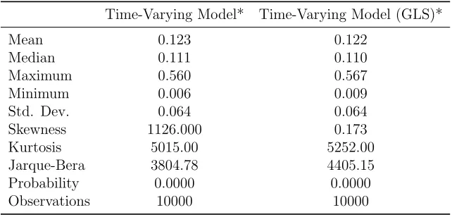
[image:22.612.144.465.465.619.2]

In this part of the paper, we estimate the model only for 5 industry portfolio using a one factor model. As the pricing errors in Equation (8) now becomes time varying as it is clear that the density will depend on the density of beta and the density of the beta will change with time. In this respect, it will become impossible to compare the results of this model with the previous two models. We only illustrate the results for the t = 1 in Table (5). Table 5: Descriptive Statistics of MCMC Chain Drawn from “Q” of Time Varying Dynamic Factor Model

Time-Varying Model* Time-Varying Model (GLS)*

Mean 0.123 0.122

Median 0.111 0.110

Maximum 0.560 0.567

Minimum 0.006 0.009

Std. Dev. 0.064 0.064

Skewness 1126.000 0.173

Kurtosis 5015.00 5252.00

Jarque-Bera 3804.78 4405.15

Probability 0.0000 0.0000

Observations 10000 10000

*Att= 1.

(23)

[image:23.612.134.555.315.621.2]

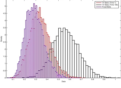
with the pricing errors of the previously estimated models, we can clearly state that the value is significantly smaller with the added dynamics for the beta. When compared with the static model, mean pricing error decreases by 33 percent and this number is bigger for dynamic factor model with fixed betas. In Figure (1), we can see how the distribution of the pricing errors changes between time-varying model and dynamic factor model with fixed betas. Lastly, to observe how the distribution of the pricing errors of time varying model changes between time=1 and time=185, we plotted the histograms of the pricing errors for these two time points and Figure (1) clearly points the shifts of the quantiles over time.

Figure 1: Histogram Plot of Mean Pricing Errors

0.1 0.2 0.3 0.4 0.5 0.6 0.7 0.8 0.9 1

0 0.5 1 1.5 2 2.5 3 3.5 4 4.5 5

Data

Density

(24)

6 Conclusion

In this paper we propose an alternative method for examining the APT pricing restrictions, using a metric first proposed byGeweke and Zhou (1996) and estimate three sets of models. Furthermore, to examine the results of such an estimation practice, we use portfolios of Fama and French that is monthly data set of 15 years grouped by industry. Utilizing Fama-French monthly portfolios and using a Bayesian methodology, we form the exact posterior distribution for the pricing errors and then calculate quantiles for the pricing error measure by estimating first a static factor model, then extending it to a dynamic factor model and lastly a dynamic model with time-varying betas. In all our models the factors are latent and all the models are estimated in one-step.

(25)

References

Aguilar, O. and M. West (2000). Bayesian dynamic factor models and portfolio allocation.

Journal of Business and Economic Statistics 18(3), 338–357.

Bai, J. and S. Ng (2002). Determining the number of factors in approximate factor models.

Econometrica 70(1), 191–221.

Blume, M. (1971). On the assessment of risk. Journal of Finance 26(1), 1–10.

Burmeister, E. and K. Wall (1986). The arbitrage pricing theory and macroeconomic factor measures. Financial Review 21(1), 1–20.

Carlin, B. and M. Cowles (1996). Markov chain monte carlo convergence diagnostics: A comparative review. Journal of the American Statistical Association 91(434), 883–904.

Chamberlain, G. (1983). Funds, factors, and diversification in arbitrage pricing models.

Chamberlain, G. and M. Rothschild (1983). Arbitrage, factor structure, and mean-variance analysis on large asset markets. Econometrica 51(5), 1281–1304.

Chen, N. (1983). Some empirical tests of the theory of arbitrage pricing. Journal of Fi-nance 38(5), 1393–1414.

Chen, N. and J. Ingersoll (1983). Exact pricing in linear factor models with finitely many assets: A note. Journal of Finance 38(3), 985–988.

Chen, N., R. Roll, and S. Ross (1986). Economic forces and the stock market. Journal of Business 59(3), 383–403.

Cochrane, J. (1996). A cross-sectional test of a production-based asset pricing model. NBER Working Paper, No:4025.

(26)

Dhrymes, P., I. Friend, and N. Gultekin (1984). A critical reexamination of the empirical evidence on the arbitrage pricing theory. Journal of Finance 39(2), 323–346.

Dybvig, P. (1983). An explicit bound on individual assets’ deviations from apt pricing in a finite economy. Journal of Financial Economics 12(4), 483–496.

Dybvig, P. and S. Ross (1985). Yes, the apt is testable.Journal of Finance 40(4), 1173–1188.

Fabozzi, F. and J. Francis (1977). Stability tests for alphas and betas over bull and bear market conditions. Journal of Finance 32(4), 1093–1099.

Faff, R., D. Hillier, and J. Hillier (2003). Time varying beta risk: An analysis of alternative modelling techniques. Journal of Business Finance and Accounting 27(5-6), 523–554.

Fama, E. and K. French (1997). Industry costs of equity. Journal of Financial Eco-nomics 43(2), 153–193.

Fama, E. and J. MacBeth (1973). Risk, return, and equilibrium: Empirical tests. Journal of Political Economy 81(3), 607–636.

Ferson, W. and C. Harvey (1991). The variation of economic risk premiums. Journal of Political Economy 99(2), 385–415.

Ferson, W. and C. Harvey (1993). The risk and predictability of international equity returns.

Review of Financial Studies 6(3), 527–566.

Ferson, W. and C. Harvey (1999). Conditioning variables and the cross section of stock returns. Journal of Finance 54(4), 1325–1360.

Ferson, W. and R. Korajczyk (1995). Do arbitrage pricing models explain the predictability of stock returns? Journal of Business 68(3), 309–349.

(27)

Geweke, J. (1992).Evaluating the Accuracy of Sampling-Based Approaches to the Calculation of Posterior Moments. Number Bayesian Statistics 4. Oxford University Press.

Geweke, J. and G. Zhou (1996). Measuring the pricing error of the arbitrage pricing theory.

The Review of financial Studies 9(2), 557–587.

Grinblatt, M. and S. Titman (1983). Factor pricing in a finite economy. Journal of Financial Economics 12(4), 497–507.

Hansen, L. (1982). Large sample properties of generalized method of moments estimators.

Harding, M. C. (2008). Explaining the single factor bias of arbitrage pricing models in finite samples. Economics Letters 99(1), 85–88.

Heidelberger, P. and P. Welch (1983). Simulation run length control in the presence of an initial transient. Operations Research 31(6), 1109–1144.

Huberman, G. (1982). A simple approach to arbitrage pricing theory. Journal of Economic Theory 28(1), 183–191.

Ingersoll, J. (1984). Some results in the theory of arbitrage pricing.Journal of Finance 39(4), 1021–1039.

King, B. (1966). Market and industry factors in stock price behavior. Journal of Busi-ness 39(1), 139–190.

Nawalkha, S. (1997). A multibeta representation theorem for linear asset pricing theories.

Journal of Financial Economics 46(3), 357–381.

Robin, A. and R. Shukla (1991). The magnitude of pricing errors in the arbitrage pricing theory. Journal of Financial Research 14(1), 65–82.

(28)

Roll, R. and S. Ross (1984). A critical reexamination of the empirical evidence on the arbitrage pricing theory: A reply. Journal of Finance 39(2), 347–350.

Ross, S. (1976). The arbitrage theory of capital asset pricing. Journal of Economic The-ory 13(3), 341–360.

Shanken, J. (1982). The arbitrage pricing theory: is it testable? Journal of Finance 37(5), 1129–1140.

Shanken, J. (1987). Multivariate proxies and asset pricing relations: Living with the roll critique. Journal of Financial Economics 18(1), 91–110.

Shanken, J. (1992a). The current state of the arbitrage pricing theory. Journal of Fi-nance 47(4), 1569–1574.

Shanken, J. (1992b). On the estimation of beta-pricing models. The Review of Financial Studies 5(1), 1–33.

Stock, J. and M. Watson (1989). New indexes of coincident and leading economic indicators.

NBER Macroeconomics Annual 4, 351–394.

Stock, J. and M. Watson (1992). A procedure for predicting recessions with leading indi-cators: Econometric issues and recent performance. Working Paper WP-92-7, Federal Reserve Bank of Chicago.

Stock, J. and M. Watson (1993). A Procedure for Predicting Recessions with Leading In-dicators: Econometric Issues and Recent Experience. Business Cycles, Indicators, and Forecasting. Chicago: The University of Chicago Press.

Tanner, M. and W. Wong (1987). The calculation of posterior distributions by data aug-mentation. Journal of the American Statistical Association 82(398), 528–540.

(29)

Appendix A

Industry Definitions

5 Industry Definition

Industry 1 Consumer Durables, NonDurables, Wholesale, Retail, and Some Services (Laundries, Repair Shops)

Industry 2 Manufacturing, Energy, and Utilities

Industry 3 Business Equipment, Telephone and Television Transmission

Industry 4 Healthcare, Medical Equipment, and Drugs

Industry 5 Other

Industry 1 Consumer NonDurables, Food, Tobacco, Textiles, Apparel, Leather, Toys

Industry 2 Consumer Durables, Cars, TV’s, Furniture, Household Appliances

Industry 3 Manufacturing, Machinery, Trucks, Planes, Chemicals, Office Furniture, Paper, Com. Printing

Industry 4 Oil, Gas, and Coal Extraction and Products

Industry 5 Business Equipment, Computers, Software, and Electronic Equipment

Industry 6 Telephone and Television Transmission

Industry 7 Wholesale, Retail, and Some Services (Laundries, Repair Shops)

Industry 8 Healthcare, Medical Equipment, and Drugs

Industry 9 Utilities

Industry 10 Other

Industry 1 Food

Industry 2 Mining and Minerals

Industry 3 Oil and Petroleum Products

Industry 4 Textiles, Apparel and Footware

Industry 5 Consumer Durables

Industry 6 Chemicals

Industry 7 Drugs, Soap, Tobacco

Industry 8 Construction and Construction Materials

Industry 9 Steel Works etc

Industry 10 Fabricated Products

Industry 11 Machinery and Business Equipment

Industry 12 Automobiles

Industry 13 Transportation

Industry 14 Utilities

Industry 15 Retail Stores

Industry 16 Banks, Insurance Companies, and Other Financials

Industry 17 Other

Appendix B

Convergence Diagnostics

Although MCMC algorithms allow an enormous expansion of the class of candidate models for a given dataset , they also suffer from a well-known potentially serious drawback: It is often difficult to decide when it is appropriate to terminate them and conclude their convergence.21 _{Almost all of the applied work involving MCMC methods has relied on}

(30)

the MCMC algorithm. Specifically, the diagnostics proposed by Heidelberger and Welch

[image:30.612.87.521.149.469.2]

(1983) and Geweke (1992) will be used.22

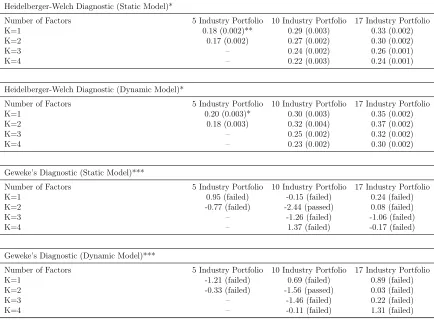
Table B.1: MCMC Diagnostic Tests for the Posterior Distribution of Q

Heidelberger-Welch Diagnostic (Static Model)*

Number of Factors 5 Industry Portfolio 10 Industry Portfolio 17 Industry Portfolio K=1 0.18 (0.002)** 0.29 (0.003) 0.33 (0.002) K=2 0.17 (0.002) 0.27 (0.002) 0.30 (0.002)

K=3 – 0.24 (0.002) 0.26 (0.001)

K=4 – 0.22 (0.003) 0.24 (0.001)

Heidelberger-Welch Diagnostic (Dynamic Model)*

Number of Factors 5 Industry Portfolio 10 Industry Portfolio 17 Industry Portfolio K=1 0.20 (0.003)* 0.30 (0.003) 0.35 (0.002) K=2 0.18 (0.003) 0.32 (0.004) 0.37 (0.002)

K=3 – 0.25 (0.002) 0.32 (0.002)

K=4 – 0.23 (0.002) 0.30 (0.002)

Geweke’s Diagnostic (Static Model)***

Number of Factors 5 Industry Portfolio 10 Industry Portfolio 17 Industry Portfolio K=1 0.95 (failed) -0.15 (failed) 0.24 (failed) K=2 -0.77 (failed) -2.44 (passed) 0.08 (failed)

K=3 – -1.26 (failed) -1.06 (failed)

K=4 – 1.37 (failed) -0.17 (failed)

Geweke’s Diagnostic (Dynamic Model)***

Number of Factors 5 Industry Portfolio 10 Industry Portfolio 17 Industry Portfolio K=1 -1.21 (failed) 0.69 (failed) 0.89 (failed) K=2 -0.33 (failed) -1.56 (passed) 0.03 (failed)

K=3 – -1.46 (failed) 0.22 (failed)

K=4 – -0.11 (failed) 1.31 (failed)

*The Cramer-von-Mises statistic to test the null hypothesis that the sampled values come from a stationary distribution. **The numbers in paranthesis stand for the p-value of the test.

**z-score for difference in means of first 10% of chain and last 50% (stationarity).