Beam Deflections: 4th Order Method and Additional Topics

(1)

11

Beam Deﬂections:

4th Order Method

and Additional Topics

(2)

Lecture 11: BEAM DEFLECTIONS: 4TH ORDER METHOD AND ADDITIONAL TOPICS

11.1. Fourth Order Method Description

The fourth-order method to find beam deflections gets its name from the order of the ODE to be integrated: E IzzvI V(x)= p(x)is a fourth order ODE. The procedure can be broken down into the

following steps.

1. Express the applied load p(x)as function of x, using positive-upward convention. This step may involve changing load signs as necessary, as in the example below.

2–3. Integrate p(x)twice to get Vy(x)and Mz(x)

4. Pause. Determine integration constants from static BCs, and replace in Mz(x). (If the constants

are too complicated when expressed in terms of the data, they might be kept in symbolic form until later.)

5–8. From here on, same as the second order method. An example of this technique follows.

§11.1.1. Example 1: Cantilever under Triangular Distributed Load

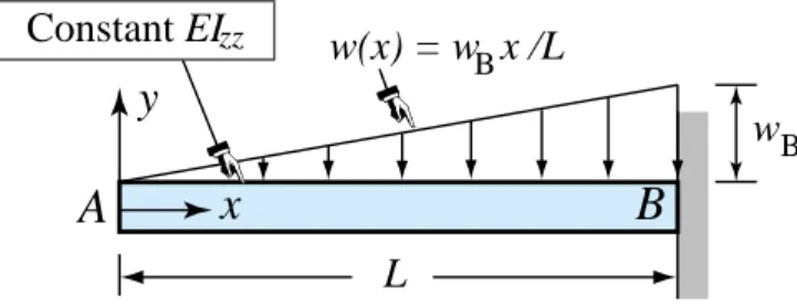
This example has been worked out in the previous lecture using the second order method. It is defined in Figure 11.1, which reproduces the figure of the previous Chapter for convenience.

w w(x) = w x /L

x

y

B B Constant EIzz

A

B

L

Figure11.1. Beam problem for Example 1. The applied loadw(x)=w_Bx/L is considered positive if it goes downward, that is, ifwB>0. This is converted to a negative load pB(x)= −wBx/L to insert in the ODEs.

From inspection the applied load is

p(x)= −wBx

L . (11.1)

Notice the minus sign to pass from the user’s convention: w(x) > 0 if directed downward, to the generic load convention: p(x) >0 if directed upward. Integrating p(x)twice yields

Vy(x)= − p(x)d x = wBx 2 2L +C1, Mz(x)= − Vy(x)d x = − wBx3 6L −C1x+C2. (11.2)

Apply now the static BCs at the free end A: Vy A =Vy(0)=C1 =0 and Mz A = Mz(0)=C2 =0.

Hence

Mz(x)= −1₂w(x)x(1₃x)= −

wBx3

(4)

Lecture 11: BEAM DEFLECTIONS: 4TH ORDER METHOD AND ADDITIONAL TOPICS P w w(x) = w x /L x y B B Constant EIzz A B

(a) Original problem

L

P

x y

A B

(b) Decomposition into two load cases and superposition

L w w(x) = w x /L x y B B A B L

=

₊

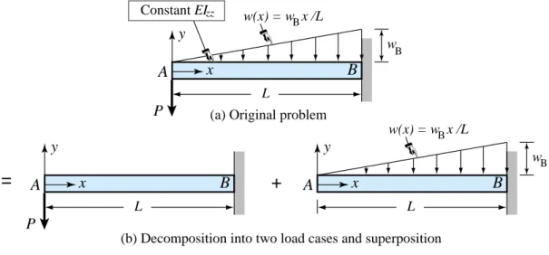
Figure11.2. Beam problem for Example 2.

From here on the steps are the same as in the second order method worked out in Lecture 10. The deflection curve is

v(x)= − wB

120E IzzL

(x5−5L4x +4L5) (11.4) The maximum deflection occurs at the cantilever tip A, and is given by

vA =v(0)= −

wBL4

30E Izz

⇓ (11.5)

The negative sign indicates that the beam deflects downward ifwB >0.

§

11.2. Superposition

All equations of the beam theory we are using are linear. This makes possible to treat complicated load cases by superposition of the solutions of simpler ones. Simple beam configurations and load cases may be compiled in textbooks and handbooks; for example Appendix D of Beer-Johnston-DeWolf. The following example illustrates the procedure.

§11.2.1. Example 2: Cantilever Under Two Load Cases

Consider the problem shown in Figure 11.2(a). The cantilever beam is subject to a tip point force as well as a triangular distributed load. This combination can be decomposed into the two load cases shown in Figure 11.2(b). Both of these have been separately solved previously as Examples 1 and 2 of Lecture 10 (the latter also as the example in the previous section). The deflection curves for these cases will be distinguished asvP(x)andvw(x), respectively.

We had obtained vP₍ x)= − P 6E Izz (L −x)2(2L +x), vw(x)= − wB 120E IzzL (x5 −5L4x+4L5) (11.6)

(5)

R w w(x) = w x /L x y B B Constant EIzz A B

(a) Original (statically indeterminate) problem

L

x y

A B

(c) Decomposition into two load cases and superposition

L w w(x) = w x /L x y B B A B L

=

₊

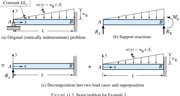
A B (b) Support reactions M A R_A R_B B

The deflection under the combined loading is obtained by adding the foregoing solutions: v(x)=vP(x)+vw(x)= − P 6E Izz (L−x)2(2L+x)− wB 120E IzzL (x5−5L4x+4L5). (11.7) The tip deflection is

vA =v(0)= − P L3 3E Izz − wBL4 30E Izz = − L3 30E Izz (10P +wBL) ⇓ (11.8)

Superposition can be also used for any other quantity of interest, for example transverse shear forces, bending moments and deflection curve slopes. An application to statically indeterminate beam analysis is given next.

§11.2.2. Example 3: A Statically Indeterminate Beam

The problem is defined in Figure 11.3(a). The beam is simply supported at A and clamped at B. If the supports are removed 3 reactions are activated: RA, RBand MB, as pictured in Figure 11.3(b).

But there are only two nontrivial static equilibrium equations: Fy = 0 and

Many poi nt = 0

becauseFx =0 is trivially satisfied. Consequently the beam is statically indeterminate because the reactions cannot be determined by statics alone. One additional kinematic equation is required to complete the analysis.

We select reaction RAas redundant force to be carried along as a fictitious applied load. Removing

the support at A and including RAmakes the beam statically determinate. See Figure 11.3(b). This

beam may be viewed as being loaded by a combination of two load cases: (1) the actual triangular loadw(x), and (2) a point load RAat A. But this is exactly the problem solved in Example 2, if we

replace P by−RA. The deflection curve of this beam is v(x)= RA 6E I (L −x) 2₍ 2L +x)− wB 120E I L(x 5₋ 5L4x +4L5). (11.9)

(6)

Lecture 11: BEAM DEFLECTIONS: 4TH ORDER METHOD AND ADDITIONAL TOPICS Now the tip deflection must be zero because there is a simple support at A. SettingvA =v(0)=0

provides the value of RA:

vA=v(0)= RAL3 3E Izz − wBL4 30E Izz = 0 ⇒ RA = wBL 10 (11.10) This reaction value can be substituted to complete the solution. For example, the bending moment is Mz(x)= RAx− wBx3 6L = wBL x 10 − wBx3 6L = wBx 30L (3L 2₋ 5x2) (11.11) The moment is zero at A (x =0), becomes positive for 0 <x < L√3/5≈.7746 L, crosses zero at x =0.7746 L and reaches Mz B = −wBL2/15 at the fixed end. The deflection is

v(x)= wB L

60E Izz

(L −x)2(2L+x)− wB

120E IzzL

(x5−5L4x +4L5), (11.12) which may be simplified to

v(x)= − wB

120 E IzzL

x(L2 −x2)2 (11.13)

§

11.3. Continuity Conditions

If the applied load is discontinuous, i.e., not a smooth function of x, it is necessary to divide the beam into segments separated by the discontinuity points. The ODEs are integrated over each segment. These solutions are “patched” by continuity conditions expressing that the slope v(x)

and the deflectionv(x)are continuous between segments. This matching results in extra relations between integration constants, which permits elimination of all integration constants except those that can be determined by the standard BCs. The procedure is illustrated with the next example. §11.3.1. Example 4: Simply Supported Beam Under Midspan Point Load

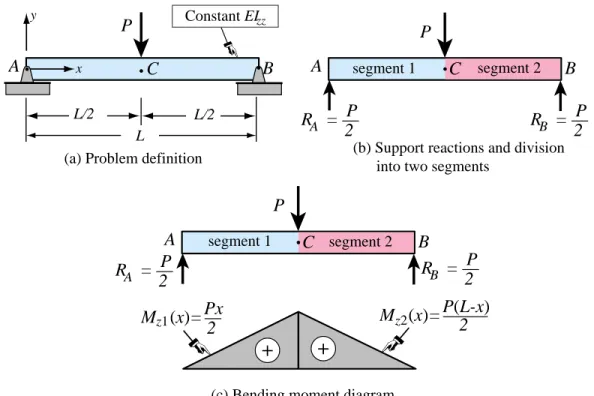
The problem is defined in Figure 11.4(a). The calculation of the deflection curve will be done by the second order method. Divide the beam into two segments: AC, which extends over 0≤x ≤ 1₂L,

and CB, which extends over 1₂L ≤ x ≤ L. For brevity, these are identified as segments 1 and 2,

respectively, in the equations below.

The expression of the bending moment over each segment is easily obtained from statics. From symmetry, the support reactions are obviously RA = RB = 1₂P as shown in Figure 11.4(b). By

inspection one obtains that the bending moment Mz(x), diagrammed in Figure 11.4(c), is

Mz(x)=   

Mz1(x)= P x₂ over segment 1 (AC), Mz2(x)= P(L−x)

2 over segment 2 (CB).

(7)

(a) Problem definition A x y C B L/2 L/2 L Constant EI_zz

(b) Support reactions and division into two segments

A B

P P

(c) Bending moment diagram

P 2 R =_A P 2 R =_B P 2 R =_A P 2 R =_B C A _B P C Px 2 M (x)=z1 P(L-x) 2 M (x)=_z2

+

segment 1 segment 1 segment 2 segment 2

Integrate Mz/E Izzover each segment:

E Izzv(x)=    E Izzv1(x)= P x 2

4 +C1 over segment 1 (AC), E Izzv₂(x)= P x(2L−x)

4 + ˆC1 over segment 2 (CB).

(11.15) It is convenient to stop here and get rid of Cˆ1 to avoid proliferation of integration constants. To

do that, note that the midspan slopev_C must be the same from both expressions: v_C =v₁(1₂L)=

v2( 1

2L). Else the beam would have a “kink” at C. This is called a continuity condition. Equating P L2/16+C1 = (3/16)P L2 + ˆC1 yields Cˆ1 = C1 − P L2/8, which is replaced in the second

expression above: E Izzv(x)=    E Izzv1(x)= P x 2

4 +C1 over segment 1 (AC), E Izzv₂(x)= P x(2L−x)

4 −

P L2

8 +C1 over segment 2 (CB).

(11.16) NowCˆ1 is gone. Integrate again both segments:

E Izzv(x)=    E Izzv1(x)= P x 3

12 +C1x+C2 over segment 1 (AC), E Izzv2(x)= P x 2₍_3L ₋_x₎ 12 − P L 2 x 8 +C1x + ˆC2 over segment 2 (CB). (11.17) To get rid of Cˆ2 we say that the midspan deflectionvC must be the same from both expressions:

(8)

Lecture 11: BEAM DEFLECTIONS: 4TH ORDER METHOD AND ADDITIONAL TOPICS yields E Izzv(x)=    E Izzv1(x)= P x 3

12 +C1x+C2 over segment 1 (AC), E Izzv2(x)= P x 2₍_3L₋_x₎ 12 − P L 2 x 8 + P L 3 48 +C1x +C2 over segment 2 (CB). (11.18) We have now only two integration constants. To determine C1and C2 use the kinematic BCs at A

and B.vA = v1(0) =C2 =0 andvB = v2(L)= 0⇒C1 = −P L2/16. Substitution gives, after

some simplifications,

E Izzv(x)=   

E Izzv1(x)= P x₄₈ (4x2−3L2) over segment 1 (AC), E Izzv2(x)= −₄₈P (4x3−12L x2+9L2x−L3) over segment 2 (CB).

(11.19) The midspan deflection, obtainable from either segment, is

vC =v1(1₂L)=v2(1₂L)= − P L3

48E Izz

(11.20) As can be seen the procedure is elaborate and error prone, even for this very simple problem. It can be streamlined by using Discontinuity Functions (DFs), which are covered in Lecture 12.