Versatile Low Power Media Access
for Wireless Sensor Networks
Joseph Polastre
Computer Science Department University of California, Berkeley
Berkeley, CA 94720 [email protected]
Jason Hill
JLH Labs 35231 Camino Capistrano Capistrano Beach, CA 92624
David Culler
Computer Science Department University of California, Berkeley
Berkeley, CA 94720 [email protected]
ABSTRACT
We propose B-MAC, a carrier sense media access protocol for wire-less sensor networks that provides a flexible interface to obtain ultra low power operation, effective collision avoidance, and high chan-nel utilization. To achieve low power operation, B-MAC employs an adaptive preamble sampling scheme to reduce duty cycle and minimize idle listening. B-MAC supports on-the-fly reconfigura-tion and provides bidirecreconfigura-tional interfaces for system services to op-timize performance, whether it be for throughput, latency, or power conservation. We build an analytical model of a class of sensor net-work applications. We use the model to show the effect of chang-ing B-MAC’s parameters and predict the behavior of sensor net-work applications. By comparing B-MAC to conventional 802.11-inspired protocols, specifically S-MAC, we develop an experimen-tal characterization of B-MAC over a wide range of network con-ditions. We show that B-MAC’s flexibility results in better packet delivery rates, throughput, latency, and energy consumption than S-MAC. By deploying a real world monitoring application with multihop networking, we validate our protocol design and model. Our results illustrate the need for flexible protocols to effectively realize energy efficient sensor network applications.
Categories and Subject Descriptors
C.2.2 [Computer-Communication Networks]: Network Proto-cols; D.4.4 [Operating Systems]: Communications Management
General Terms
Performance, Design, Measurement, Experimentation
Keywords
Wireless Sensor Networks, Media Access Protocols, Energy Effi-cient Operation, Reconfigurable Protocols, Networking, Commu-nication Interfaces.
Permission to make digital or hard copies of all or part of this work for personal or classroom use is granted without fee provided that copies are not made or distributed for profit or commercial advantage and that copies bear this notice and the full citation on the first page. To copy otherwise, to republish, to post on servers or to redistribute to lists, requires prior specific permission and/or a fee.
SenSys’04, November 3–5, 2004, Baltimore, Maryland, USA.
Copyright 2004 ACM 1-58113-879-2/04/0011 ...$5.00.
1.
INTRODUCTION
In wireless sensor network deployments, reliably reporting data while consuming the least amount of power is the ultimate goal. One such application that drives the design of low power media ac-cess control (MAC) protocols is environmental monitoring. Main-waring et. al. [12] and the UCLA Center for Embedded Network Sensing [2, 6] have deployed wireless sensors for microclimate monitoring that operate at low duty cycles with multihop network-ing and reliable data reportnetwork-ing. They show that MAC mechanisms must support duty cycles of 1% while efficiently transferring var-ious workloads and adapting to changing networking conditions. These workloads include periodic data reporting, bulk log transfer, and wirelessly reprogramming a node. In this paper we discuss the design of a MAC protocol motivated by monitoring applications.
Nodes in a wireless sensor network do not exist in isolation; rather they are embedded in the environment, causing network links to be unpredictable [16]. As the surrounding environment changes, nodes must adjust their operation to maintain connectivity. For ex-ample, RF performance may be hindered by a sudden rain storm or the opening and closing of doors in a building.
Woo [21] and Zhao [24] have studied the volatility in link qual-ity in wireless sensor networks. Zhao shows the existence of “gray areas” where some nodes exceed 90% successful reception while neighboring nodes receive less than 50% of the packets. He shows that the gray area is rather large–one-third of the total communica-tion range. Woo independently verified Zhao’s gray area findings. In designing a reliable multihop routing protocol, Woo shows that effectively estimating link qualities is essential. Snooping on traf-fic over the broadcast medium is crucial for extracting information about the surrounding topology. By snooping, network protocols can prevent cycles, notify neighboring nodes of unreachable routes, improve collision avoidance, and provide link quality information. Since data must ultimately be reported out of the network, the me-dia access protocol must be flexible to meet changing network pro-tocol demands.
Not only are the networking conditions different, applications for wireless sensor networks have different demands than those de-signed for traditional ad-hoc wireless networks. Intanagonwiwat et. al. [8] show how 802.11 is inappropriate for low duty cycle sensor network data delivery. Idle listening in 802.11 consumes as much energy when the protocol is idle as it does when receiving data. Idle listening occurs when a node is active, but there is no meaningful activity on the channel resulting in wasted energy. is no activity. It is absolutely crucial that the MAC protocol support a duty cycling mechanism to eliminate idle listening.
community, data must flow from the network predictably and reli-ably. Scientists determine the sample period and physical deploy-ment of the nodes. The role of the network is to ensure that data is delivered as expected. A general rule for achieving predictable operation is to reduce complexity as much as possible from the application and its services. Since each node executes a single ap-plication, it is important to optimize communication performance for that application–not for a generic set of users.
To meet the requirements of wireless sensor network deploy-ments and monitoring applications, we translate them to a set of goals for the media access protocol. Our goals for a MAC protocol for wireless sensor network applications are:
• Low Power Operation • Effective Collision Avoidance
• Simple Implementation, Small Code and RAM Size • Efficient Channel Utilization at Low and High Data Rates • Reconfigurable by Network Protocols
• Tolerant to Changing RF/Networking Conditions • Scalable to Large Numbers of Nodes
To meet these goals, we propose B-MAC, a configurable MAC protocol for wireless sensor networks. It is simple in both design and implementation. It has a small core and factors out higher layer functionality. Factoring out some functionality and exposing con-trol to higher services allows the MAC protocol to support a wide variety of sensor network workloads. This minimalist model of MAC protocol design is in contrast to the classic monolithic MAC protocols optimized for a general set of workloads; however this paper shows the effectiveness of a small, configurable MAC proto-col that supports low duty cycle applications.
The contributions of this paper are not only the design of a ver-satile MAC protocol for sensor networks. We propose an adaptive bidirectional interface for wireless sensor network applications. The interface allows middleware services to reconfigure the MAC pro-tocol based on the current workload. We build a model of appli-cation performance that may be used to reconfigure B-MAC and maximize a node’s lifetime. We use a comprehensive set of mi-crobenchmarks to experimentally characterize wireless sensor net-work (WSN) performance. To validate the model, we built an en-vironmental monitoring application and show how its performance matches our model’s predictions. Our model can be used to iden-tify the best parameters for an arbitrary low power wireless sensor network application at compile or run time and estimate the ap-plication’s lifetime. We illustrate the importance of reconfiguration through simple optimizations that extend network lifetime by 50%.
2.
RELATED WORK
Most MAC protocols for wireless sensor networks have been based on conventional wireless protocols, especially 802.11. These protocols typically provide a general purpose mechanism that works reasonably well for a large set of traffic workloads. The previous efforts serve as building blocks for designing a MAC protocol that meets our goals.
The DARPA Packet Radio Network (PRNET) [10] was one of the first ad-hoc multihop wireless networks. PRNET had two me-dia access protocols–Slotted ALOHA [1] and Carrier Sense Multi-ple Access [9]. Much of the standard MAC protocol functionality– including random delays, forwarding delays, link quality estima-tion, and low duty cycle through node synchronization–were first
executed in PRNET. CSMA is validated as a way to efficiently use the majority of the channel’s bandwidth while duty cycling nodes. TDMA and slotted ALOHA solutions in PRNET were ultimately dismissed due to their inability to scale.
Woo and Culler [20] illustrate the effect of changing the MAC protocol based on the workload. They show that sensor network application scenarios and network traffic characteristics differ sig-nificantly from conventional computer networks. Typically data is sent periodically in short packets. To achieve fairness and energy efficient transmission through a multihop network, they design an adaptive rate control protocol to that is optimized forn-to-1data reporting and multihop networking. Existing MAC protocols are simply not suitable due to their failure to efficiently support sensor network workloads in low duty cycle conditions.
Hill and Culler [7] demonstrate a form of preamble sampling to reduce idle listening cost. In Hill’s RF wakeup scheme, the analog baseband of the radio is sampled for energy every 4 seconds. By quickly evaluating the channel’s energy, he reduced the duty cycle of the radio to below 1%. He demonstrated the use of low power RF wakeup on an 800 node multihop network. The ASK radio used by Hill allows very brief radio sampling; we develop a related technique that works on more complex radios.
Published concurrently with Hill’s work, Aloha with preamble sampling [4] presents a low power technique similar to that used in paging systems [13]. To let the receiver sleep for most of the time when the channel is idle, nodes periodically wake up and check for activity on the channel. If the channel is idle, the receiver goes back to sleep. Otherwise, the receiver stays on and continues to listen until the packet is received. Packets are sent with long preambles to match the channel check period. El-Hoiydi [4] creates a model for Aloha with preamble sampling and presents the effect of delay due to long preambles. He proposes using the long preamble for initial synchronization of nodes; afterwards the nodes transmit and receive on a schedule with normal sized packets.
WiseMAC [5] is an iteration on Aloha with preamble sampling specifically designed for infrastructure wireless sensor networks. The main contribution of WiseMAC is an evaluation of the power consumption of WiseMAC, 802.11, and 802.15.4 under low traffic loads. They show that for the same delay, WiseMAC and pream-ble sampling lowered power consumption by 57% over PSM used in 802.11 and 802.15.4. WiseMAC meets many of our goals ex-cept that it has no mechanism to reconfigure based on changing demands from services using the protocol.
S-MAC [22] is a low power RTS-CTS protocol for wireless sen-sor networks inspired by PAMAS [15] and 802.11. S-MAC peri-odically sleeps, wakes up, listens to the channel, and then returns to sleep. Each active period is of fixed size, 115 ms, with a vari-able sleep period. The length of the sleep period dictates the duty cycle of S-MAC. At the beginning of each active period, nodes ex-change synchronization information. Following the SYNC period, data may be transferred for the remainder of the active period us-ing RTS-CTS. In a follow up paper [23], the authors add adaptive listening–when a node overhears a neighbor’s RTS or CTS packets, it wakes up for a short period of time at the end of their neighbor’s transmission to immediately transmit its own data. By changing the duty cycle, S-MAC can trade off energy for latency. S-MAC includes a fragmentation mechanism that uses RTS-CTS to reserve the channel, then transmits packets in a burst. Although S-MAC achieves low power operation, it does not meet our goals of sim-ple imsim-plementation, scalability, and tolerance to changing network conditions. As the size of the network increases, S-MAC must maintain an increasing number of neighbors’ schedules or incur additional overhead through repeated rounds of resynchronization.
interface MacControl {
command result_t EnableCCA(); command result_t DisableCCA(); command result_t EnableAck(); command result_t DisableAck(); command void* HaltTx(); }
interface MacBackoff {
event uint16_t initialBackoff(void* msg); event uint16_t congestionBackoff(void* msg); }
interface LowPowerListening {
command result_t SetListeningMode(uint8_t mode); command uint8_t GetListeningMode();
command result_t SetTransmitMode(uint8_t mode); command uint8_t GetTransmitMode();
command result_t SetPreambleLength(uint16_t bytes); command uint16_t GetPreambleLength();
command result_t SetCheckInterval(uint16_t ms); command uint16_t GetCheckInterval();
}
Figure 1: Interfaces for flexible control of B-MAC by higher layer services. These TinyOS interfaces allow services to tog-gle CCA and acknowledgments, set backoffs on a per message basis, and change the LPL mode for transmit and receive.
T-MAC [19] improves on S-MAC’s energy usage by using a very short listening window at the beginning of each active period. After the SYNC section of the active period, there is a short window to send or receive RTS and CTS packets. If no activity occurs in that period, the node returns to sleep. By changing the protocol to have an adaptive duty cycle, T-MAC saves power at a cost of reduced throughput and additional latency. T-MAC, in variable workloads, uses one fifth the power of S-MAC. In homogeneous workloads, T-MAC and S-T-MAC perform equally well. T-T-MAC suffers from the same complexity and scaling problems of S-MAC. Shortening the active window in T-MAC reduces the ability to snoop on surround-ing traffic and adapt to changsurround-ing network conditions.
Many of these protocols have only been evaluated in simulation. Not only must the protocol perform well in simulation, it must also integrate well with the implementation of wireless sensor network applications. Each of the protocols described in this section provide solutions that meet a subset of our goals. Motivated by monitoring applications for wireless sensor networks, we build upon ideas from previously published work to create a reconfigurable protocol that meets all of the goals from Section 1.
3.
DESIGN AND IMPLEMENTATION
To achieve the goals outlined in Section 1, we designed a CSMA protocol for wireless sensor networks called B-MAC, Berkeley Me-dia Access Control for low power wireless sensor networks. Al-though B-MAC is motivated by the needs of monitoring applica-tions, the flexibility of our protocol allows allows other services and applications to be realized efficiently. These services include, but are not limited to, target tracking, localization, triggered event reporting, and multihop routing.
Classical MAC protocols perform channel access arbitration and are tuned for good performance over a set of workloads thought to be representative of the domain. S-MAC is an example of a wireless sensor network protocol designed using a classical ap-proach. S-MAC provides an RTS-CTS mechanism for channel ar-bitration and hidden terminal avoidance, synchronization with its
0 20 40 60 80 100
110 100 90 80
si
gn
al
(d
B
m
)
0 20 40 60 80 100
0 1
Th
re
sh
ol
d
0 20 40 60 80 100
0 1
Time (ms)
O
ut
lie
r
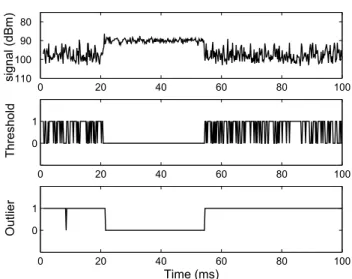
Figure 2: Clear Channel Assessment (CCA) effectiveness for a typical wireless channel. The top graph is a trace of the received signal strength indicator (RSSI) from a CC1000 transceiver. A packet arrives between 22 and 54ms. The middle graph shows the output of a thresholding CCA algorithm. 1indicates the channel is clear,0indicates it is busy. The bottom graph shows the output of an outlier detection algorithm.
neighbors for low power operation, and message fragmentation for efficiently transferring bulk data. S-MAC is not only a link proto-col, but also network and organization protocol. Applications and services must rely on S-MAC’s internal policies to adjust its op-eration as node and network conditions change; such changes are opaque to the application. In contrast, the B-MAC protocol con-tains a small core of media access functionality. B-MAC uses clear channel assessment (CCA) and packet backoffs for channel arbitra-tion, link layer acknowledgments for reliability, and low power lis-tening (LPL) for low power communication. B-MAC is only a link protocol, with network services like organization, synchronization, and routing built above its implementation. Although B-MAC nei-ther provides multi-packet mechanisms like hidden terminal sup-port or message fragmentation nor enforces a particular low power policy, B-MAC has a set of interfaces that allow services to tune its operation (shown in Figure 1) in addition to the standard message interfaces1. These interfaces allow network services to adjust
B-MAC’s mechanisms, including CCA, acknowledgments, backoffs, and LPL. By exposing a set of configurable mechanisms, protocols built on B-MAC make local policy decisions to optimize power consumption, latency, throughput, fairness or reliability.
For effective collision avoidance, a MAC protocol must be able to accurately determine if the channel is clear, referred to as Clear Channel Assessment (CCA). Since the ambient noise changes de-pending on the environment, B-MAC employs software automatic gain control for estimating the noise floor. Signal strength samples are taken at times when the channel is assumed to be free–such as immediately after transmitting a packet or when the data path of the radio stack is not receiving valid data. Samples are then en-tered into a FIFO queue. The median of the queue is added to an exponentially weighted moving average with decayα. The median is used as a simple low pass filter to add robustness to the noise 1Standard interfaces for message transmission in TinyOS [18] are BareSendMsg for transmission, ReceiveMsg for reception, andRadioCoordinatorfor time stamping and start of frame delimiter (SFD) information.
0 0.5 1 1.5 2 2.5 3 0
5
10
15
20
25
30
Time (ms)
Curr
e
nt
(m
A
)
(a) (b) (c) (d) (e) (f) (g) sleep initradio radio crystal startup µc rx adc sleep
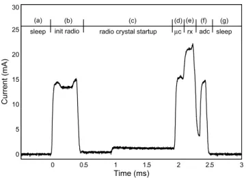
Figure 3: When turning on the radio, the node must perform a sequence of operations. The node first starts in sleep state (a), then wakes up on a timer interrupt (b). The node initial-izes the radio configuration and commences the radio’s startup phase. The startup phase (c) waits for the radio’s crystal oscil-lator to stabilize. Upon stabilization, the radio enters receive mode (d). After the receive mode switch time, the radio enters receive mode (e) and a sample of the received signal energy may begin. After the ADC starts acquisition, the radio is turned off and the ADC value is analyzed (f). With LPL, if there is no activity on the channel, the node returns to sleep (g).
floor estimate. Anαvalue of0.06and FIFO queue size of10 pro-vided the best results for a typical wireless channel. Once a good estimate of the noise floor is established, a request to transmit a packet starts the process of monitoring the received signal from the radio. A common method used in a variety of protocols, including 802.15.4, takes a single sample and compares it to the noise floor. This thresholding method produces results with a large number of false negatives that lower the effective channel bandwidth. Since noise has significant variance in channel energy whereas packet re-ception has fairly constant channel energy (as shown in Figure 2), B-MAC searches for outliers in the received signal such that the channel energy is significantly below the noise floor. If an out-lier exists during the channel sampling period, B-MAC declares the channel is clear since a valid packet could never have an outlier significantly below the noise floor. If five samples are taken and no outlier is found, the channel is busy. The effectiveness of outlier de-tection as compared to thresholding on a trace from a CC1000 [3] transceiver is shown in Figure 2.
The most basic mechanism allows services to turn CCA on or off using theMacControlinterface in Figure 1. By disabling CCA, a scheduling protocol may be implemented above B-MAC. If CCA is enabled, B-MAC uses an initial channel backoff when sending a packet. B-MAC does not set the backoff time, instead an event is signaled to the service that sent the packet via theMacBackoff interface. The service may either return an initial backoff time or ignore the event. If ignored, a small random backoff is used. After the initial backoff, the CCA outlier algorithm is run. If the channel is not clear, an event signals the service for a congestion backoff time. If no backoff time is given, again a small random backoff is used. Enabling or disabling CCA and configuring the backoff allows services to change the fairness and available throughput.
B-MAC provides optional link-layer acknowledgment support. If acknowledgments are enabled, B-MAC immediately transfers an
acknowledgment code after receiving a unicast packet. If the trans-mitting node receives the acknowledgment, an acknowledge bit is set in the sender’s transmission message buffer.
B-MAC duty cycles the radio through periodic channel sampling that we call Low Power Listening (LPL). Our technique is similar to preamble sampling in Aloha [4] but tailored to different radio characteristics. Each time the node wakes up, it turns on the ra-dio and checks for activity. If activity is detected, the node powers up and stays awake for the time required to receive the incoming packet. After reception, the node returns to sleep. If no packet is received (a false positive), a timeout forces the node back to sleep. Accurate channel assessment (CCA) is critical to achieving low power operation with this method. We use the noise floor estima-tion of B-MAC not only for finding a clear channel on transmission but also for determining if the channel is active during LPL. False positives in the CCA algorithm (such as those caused by thresh-olding) severely affect the duty cycle of LPL due to increased idle listening.
To reliably receive data, the preamble length is matched to the interval that the channel is checked for activity. If the channel is checked every 100 ms, the preamble must be at least 100 ms long for a node to wake up, detect activity on the channel, receive the preamble, and then receive the message. Idle listening occurs when the node wakes up to sample the channel and there is no activity. The interval between LPL samples is maximized so that the time spent sampling the channel is minimized. The check interval and preamble length are examples of parameters exposed through B-MAC’sLowPowerListeninginterface in Figure 1. Transmit mode corresponds to the preamble length and the listening mode corresponds to the check interval. We provide a selection of 8 dif-ferent modes (corresponding to 10, 20, 50, 100, 200, 400, 800, and 1600ms for the check interval). Protocols may also set their own preamble length and check interval through the interface. The ef-fect of varying the preamble size and check interval is discussed in more detail in Section 4. Examples of services that use the LPL interface are given in Subsection 4.3 and Section 8.
A trace of the power consumption while sampling the channel on a Mica2 mote [17] is shown in Figure 3. The process in Figure 3 applies to essentially any MAC protocol for sensor networks. It performs initial configuration of the radio (b), starts the radio and its oscillator (c), switch the radio to receive mode (d), and then per-form the actions of the protocol. As a result, the cost for powering up the radio is the same for all protocols. The difference between protocols is how long the radio is on after it has been started and how many times the radio is started.
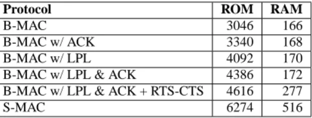
In sensor networks, each node typically runs a single applica-tion. Since the RAM and ROM available on sensor nodes are ex-tremely limited, keeping the size of the MAC implementation small is important. Reducing the complexity of the protocol reduces state and the likelihood of race conditions We implemented B-MAC in TinyOS [11] to evaluate its efficacy in meeting our goals. Since B-MAC does not have the RTS-CTS mechanism or synchronization requirements of S-MAC2, the implementation is both simpler and
smaller as shown in Table 1. B-MAC does not hinder efficient im-plementation of network protocols; above B-MAC we implemented an RTS-CTS scheme and a message fragmentation service using B-MAC’s control interfaces that have equivalent functionality to S-MAC RTS-CTS and fragmentation services.
2
All tests with S-MAC were performed with the implementa-tion in tinyos-1.x/contrib/s-mac/in the TinyOS CVS repository [18] as of March 30, 2004. The B-MAC implemen-tation for the Mica2 is located in the TinyOS CVS repository at tinyos-1.x/contrib/ucb/tos/lib/CC1000Pulse/.
Protocol ROM RAM
B-MAC 3046 166
B-MAC w/ ACK 3340 168
B-MAC w/ LPL 4092 170
B-MAC w/ LPL & ACK 4386 172
B-MAC w/ LPL & ACK + RTS-CTS 4616 277
S-MAC 6274 516
Table 1: A comparison of the size of B-MAC and S-MAC in bytes. Both protocols are implemented in TinyOS.
4.
CONCEPTS AND TRADEOFFS
In this section we describe a framework for analyzing the oper-ation of a wireless sensor network applicoper-ation. We build an ana-lytical model for monitoring applications. The model allows us to calculate and set B-MAC’s parameters to optimize the application’s overall power consumption. Using the model, we illustrate the ef-fect of different application variables including duty cycle, network density, and sampling rate. We show how B-MAC’s interfaces may be used by network services to adapt to current demands.
4.1
Modeling Lifetime
To calculate node duty cycle and lifetime, we examine a periodic sensing application (such as in [12]) that streams sensor data to a base station. Table 2 lists the primitive operations performed by a low power monitoring application and the observed costs when using a CC1000 transceiver. These operations describe a represen-tative class of radios for wireless sensor networks. Radios with similar properties are manufactured by Chipcon, Infineon, and Mo-torola. We use the notation and values in Table 2 throughout the remainder of this paper.
The node’s lifetime is determined by its overall energy consump-tion. If the lifetime is maximized, then the energy consumption must be minimized. All of the energies,E, are defined in units of millijoules per second, or milliwatts. Calculating the total energy usage can be done by multiplyingEby the node lifetimetl. For wireless sensor network applications, the energy used by a node consists of the energy consumed by receiving, transmitting, listen-ing for messages on the radio channel, sampllisten-ing data, and sleeplisten-ing.
E=Erx+Etx+Elisten+Ed+Esleep (1)
Sensors are an integral part of wireless sensor networks and must be considered when calculating a node’s lifetime. Sampling sen-sors is often expensive and affects the lifetime of the node. The sampling parameters (shown in Table 2) are based on an applica-tion deployed by Mainwaring et. al. [12]. In their applicaapplica-tion, each node takes 1100 ms to start its sensors, sample, and collect data. The data is sampled every five minutes, orr = 1/(5∗60). The energy associated with sampling data,Ed, is
td=tdata×r
Ed=tdcdataV (2) The energy consumed by transmitting,Etx, is simply the length of the packet with the preamble times the rate packets are generated by the application.
ttx=r×(Lpreamble+Lpacket)ttxb
Etx=ttxctxbV (3)
For a periodic application with a uniform sampling rate, the node will detect and receive data when each of itsnneighbors transmit
Operation Time (s) I (mA)
Initialize radio (b) 350E-6 trinit 6 crinit Turn on radio (c) 1.5E-3 tron 1 cron Switch to RX/TX (d) 250E-6 trx/tx 15 crx/tx Time to sample radio (e) 350E-6 tsr 15 csr Evaluate radio sample (f) 100E-6 tev 6 cev
Receive 1 byte 416E-6 trxb 15 crxb
Transmit 1 byte 416E-6 ttxb 20 ctxb
Sample sensors 1.1 tdata 20 cdata
Table 2: Time and current consumption (I) for completing primitive operations of a monitoring application using the Mica2 mote and CC1000 transceiver. Identifiers on each op-eration map back to the activities of acquiring a radio sample in Figure 3.
Notation Parameter Default
csleep Sleep Current (mA) 0.030
Cbatt Capacity of battery (mAh) 2500
V Voltage 3
Lpreamble Preamble Length (bytes) 271
Lpacket Packet Length (bytes) 36
ti Radio Sampling Interval (s) 100E-3
n Neighborhood Size (nodes) 10
r Sample Rate (packets/s) 1/300
tl Expected Lifetime (s)
-Table 3: Parameters for a monitoring application running B-MAC. The first three parameters are specific to Mica2 motes; the next three are default values for B-MAC parameters on the Mica2; the remaining parameters are application seman-tics affecting B-MAC’s performance. Each parameter affects the node’s total energy consumption,E.
a packet, regardless of the packet’s destination. We refer to the density of neighbors surrounding a node as the neighborhood size of the node. Although receiving data from neighbors shortens a node’s lifetime, it allows services to snoop on the channel and make decisions based on channel activity.
We can bound the total time the node will spend receiving and calculate an upper bound on the energy consumed by receiving, Erx.
trx≤nr(Lpreamble+Lpacket)trxb
Erx=trxcrxbV (4)
Our analysis is based on a single cell. To analyze a multihop application, we need to account for the routing traffic through each node due to its children and its neighbors’ children. Instead ofr packets per second flowing through a particular node, the traffic through the node must also include all the packets routed by the node and its neighbors. The function children(i) is defined by the multihop routing protocol.
r× n X
i=0
(children(i) + 1)
Up to this point, our model has been independent of the MAC protocol in use. The MAC protocol is responsible for minimiz-ing idle listenminimiz-ing time, tlisten. In B-MAC, idle listening occurs whenever B-MAC samples the channel for activity but no activity is present.
0 20 40 60 80 100 0
20 40 60 80 100 120 140 160 180 200
Neighborhood size
Channel Activity Check Interval (ms)
0.25
0.5 0.75 1 1.25 1.5
2
2.5
Figure 4: Contour of node lifetime (in years) based on LPL check time and network density. If both parameters are known, their intersection is the expected lifetime using the optimal B-MAC parameters.
In order to reliably receive packets, the LPL check interval,ti, must be less than the time of the preamble. Therefore we have the constraint:
Lpreamble≥ dti/trxbe
Given a check interval and associated preamble length, we can calculate the time spent sampling the channel. From Figure 3, the power consumption of a single LPL radio sample is17.3µJ. The total energy spent listening to the channel is the energy of a single channel sample times the channel sampling frequency.
Esample= 17.3µJ
tlisten= (trinit+tron+trx/tx+tsr)×
1 ti
Elisten≤Esample×
1
ti (5)
Finally, the node must sleep for the remainder of the time. The sleep time,tsleep, is simply the time remaining each second that’s not consumed by other operations.
tsleep= 1−trx−ttx−td−tlisten
Esleep=tsleepcsleepV (6)
The lifetime of the node, tl, is dependent on the total energy consumed,E, and the battery capacity,Cbatt. We must bound the lifetime by the available capacity of the battery.
tl=
Cbatt×V
E ×60×60 (7)
By solving the system of equations (1 through 6) and entering the parameters in Table 3, we can find the minimum energy for a given network configuration. Lifetime may be estimated at compile time, or computed for a discrete set of values at runtime that provides reconfiguration feedback to network services.
0 20 40 60 80 100
0 1 2 3 4 5 6 7 8 9 10
Number of neighboring nodes
Effective duty cycle (%)
200ms check interval 100ms check interval 50ms check interval 25ms check interval 10ms check interval
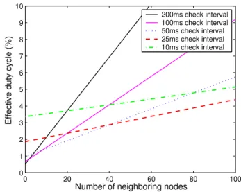
Figure 5: The node’s duty cycle is affected by the network den-sity and LPL check interval. Typically used LPL check inter-vals in B-MAC’s implementation are depicted. The best check interval is the lowest line at a given network density.
4.2
Parameters
In a typical deployment, scientists will determine the physical location of the nodes (which affects each node’s neighborhood size, n) and the ideal sampling rate,r. With this information, we can calculate the parameters to attain the best lifetime that B-MAC can achieve. This also provides the scientist with an estimate for how long the network will live.
If we fix the sample rate and vary the network density,n, we can evaluate the affect of neighbors on node lifetime. Solving the system of equations from this section with the sample rate equal to once every five minutes yields Figure 4. Taking a few slices across the figure at realistic check intervals is shown in Figure 5. To find the best LPL check interval for an application, find the expected neighborhood size in Figure 5 and move up the y-axis to the low-est line. The check interval corresponding with this line will yield the maximum lifetime. For example, a check interval of 50 ms is optimal for a neighborhood size of 20, but if the neighborhood size is only 5, a check interval of 100 ms is optimal. The size of the neighborhood affects the amount of traffic flowing by each node. B-MAC trades off idle listening for a reduced time to transmit and receive.
If we assume we have a network with approximately 10 neigh-bors per node, the optimum LPL check interval changes with sam-ple rate. Increasing the samsam-ple rate increases the amount of traffic in the network (just as increasing the neighborhood size also in-creases the traffic in a periodic application). As a result, each node overhears more packets. We must find the optimal check interval tisuch that we maximize the lifetimetl. Loweringtialso lowers the preamble length. The time to transmit and receive a packet is shorter and the radio is sampled more often.
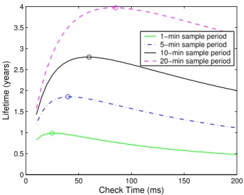
The tradeoff of more frequently checking the radio in order to shorten the packet transmission time is shown in Figure 6. Notice that the penalty for more idle listening than required by the traffic pattern, left of the maximum lifetime point in Figure 6, is much more severe than the penalty for sending packets that are longer than necessary.
0 50 100 150 200 0
0.5 1 1.5 2 2.5 3 3.5 4
Check Time (ms)
Lifetime (years)
1−min sample period 5−min sample period 10−min sample period 20−min sample period
Figure 6: The lifetime of each node is dependent on the check interval and the amount of traffic in the network cell. Each line shows the lifetime of the node at that sample rate and LPL check interval. The circles occur at the maximum lifetime (op-timal check interval) for each sample rate.
4.3
Adaptive Control
Our model shows that it is advantageous to change the parame-ters of the MAC protocol based on changing network conditions. Since sensor networks consist of low power volatile nodes, it is likely that links will appear or disappear over time [21, 24]. Nodes may join and leave the network, or the size of the neighborhood will change due to changes in the physical environment. The MAC protocol must be able to adjust for these changes and optimize its power consumption, latency, and throughput to support the services relying on it. The analytical model allows the node to recompute the check interval and preamble length. To address reconfiguration, we chose not to implement the functionality in the MAC protocol as Woo and Culler [20] have done. Instead, we created a set of bidi-rectional interfaces that allow services to change the MAC protocol based on their current operating conditions.
By factoring out more complex parts of conventional MAC pro-tocols, services can decide which situations warrant the use of addi-tional control. For example, B-MAC’s link layer acknowledgment support may be selected on a per-packet basis. When an acknowl-edgment fails, services may choose to retransmit the packet, change the packet’s destination, or reconfigure the LPL parameters.
One scheme implemented above B-MAC is an RTS-CTS channel acquisition protocol. On each packet transmission, an RTS packet is sent. A CTS response is sent if the destination node is idle and not delaying due to other transmissions. The RTS and CTS pack-ets are sent using LPL. Once the channel is acquired, data and ac-knowledge packets are sent immediately with CCA and LPL dis-abled. After acknowledgment, both nodes reenable LPL and CCA, then they return to sleep.
5.
EXPERIMENTAL METHOD
To illustrate the effectiveness of a lightweight, configurable MAC protocol, we compare B-MAC to existing MAC protocols, specif-ically S-MAC and T-MAC. Each protocol is run through a set of simple workloads forming an empirical characterization of pro-tocol performance. The purpose of these microbenchmarks is to show how WSN protocols react to typical wireless sensor network
Length (bytes) B-MAC S-MAC
Preamble 8 18
Synchronization 2 2
Header 5 9
Footer (CRC) 2 2
Data Length 29 29
Total 46 60
Table 4: B-MAC and S-MAC as implemented in TinyOS have different protocol overhead when sending a data packet. S-MAC has a larger header to accommodate timestamp infor-mation. The data payload is the default payload for TinyOS applications; however, both B-MAC and S-MAC send only the length specified by higher level services.
conditions–high contention, low to high throughput, low to high la-tency, and their correlation with power consumption. We contrast the use of RTS-CTS and message fragmentation services imple-mented using B-MAC’s interfaces to the same mechanisms that are part of the S-MAC protocol. These microbenchmarks build an un-derstanding of how a real application would perform. To validate the model in Section 4, we look in detail at the performance of a deployed monitoring application that uses B-MAC. We compare the actual node duty cycles with those predicted by our model and show that our empirical characterizations apply to real world appli-cations.
Both B-MAC and S-MAC were implemented in TinyOS. We used the Mica2 [17] wireless sensor nodes to perform our tests. All tests occurred in an unobstructed area with line of sight to ev-ery other node. To enable multihop networking, we reduced the RF output power of the node to its minimum value and placed the nodes with 1 meter spacing. Nodes were elevated 15 centimeters to reduce near-field effects.
To determine the power consumption of each protocol, we im-plemented counters in the MAC protocol that keep track of how many times various operations were performed. For B-MAC, this includes receiving a byte, transmitting a byte, and checking the channel for activity. For S-MAC, we count the amount of time that the node is active, number of bytes transmitted and received, and the additional time the node spent awake due to adaptive listening. Since the S-MAC implementation does not actually put the node into sleep mode, we had to measure the power consumption in-directly by multiplying the cumulative time of each operation with the expected power to operate in that mode. All of our data assumes that S-MAC actually enters sleep mode even though the implemen-tation does not. The power consumption of each operation is taken from Table 2.
In addition to tests on real sensor network hardware, we simu-lated T-MAC [19] in Matlab. We calcusimu-lated the time of each opera-tion and multiplied by the current consumpopera-tion in Table 2 to get the overall expected power consumption of the T-MAC protocol. At the time of our experiments, there was no TinyOS implementation of T-MAC available to do a direct comparison between B-MAC, S-MAC, and T-MAC.
To measure latency, each node is connected to an oscilloscope. Upon submission of a packet to the MAC protocol, we toggle a hardware pin. When a packet is received, a different pin is tog-gled. Using an oscilloscope, we capture the time between each pin toggling to yield the total latency.
In some graphs we show the optimal solution. Found by com-puting a perfect schedule, the optimal solution is the minimum
to-0 5 10 15 20 0
2000 4000 6000 8000 10000 12000 14000 16000
0 5 10 15 200
0.1 0.2 0.3 0.4 0.5 0.6 0.7 0.8 0.9 1
Number of nodes
Percentage of Channel Capacity
B−MAC B−MAC w/ ACK B−MAC w/ RTS−CTS S−MAC unicast S−MAC broadcast Channel Capacity
Throughput (bps)
Figure 7: Measured throughput of each protocol with no duty cycle under a contended channel. The throughput of each pro-tocol is affected by the amount of nodes contending for the channel and the protocol’s overhead. B-MAC achieves over 4.5 times the throughput of the standard S-MAC unicast protocol through lower per-packet processing and effective CCA.
tal transmit and receive costs possible. In this solution, all nodes are perfectly synchronized with no additional overhead. This met-ric serves to show the effect of overhead in sensor network MAC protocols. To calculate the power consumption, the transmit and receive times are multiplied by the power to perform those opera-tions.
In all cases, we measure the data throughput of the network. This factors out the protocol-specific overhead to evaluate the amount of data that can be delivered by each protocol and the cost of deliver-ing that data. In all tests where we mention “packet size”, we are referring to the size of the data payload only, not the header infor-mation. The overhead attributed to each protocol is shown in Ta-ble 4. S-MAC uses a longer preamTa-ble and contains time stamping information in the header. Note that control and synchronization packets in S-MAC are 10 bytes long plus preamble and synchro-nization (total 30 bytes). For some tests, we vary the data length. Table 4 shows the default data lengths; however both B-MAC and S-MAC only transmit the data length specified by the application on a per packet basis.
6.
MICROBENCHMARK ANALYSIS
In this section we use a variety of microbenchmarks to show how B-MAC’s functionality may be used effectively. These benchmarks show the effect of a wide array of network conditions on the energy consumption of B-MAC, S-MAC, and T-MAC. We show the po-tency of B-MAC’s interfaces for building efficient applications and communications protocols. The results of the microbenchmarks empirically characterize the performance of B-MAC, providing in-sight on B-MAC’s expected behavior in real world applications.
6.1
Channel Utilization
Channel utilization is a traditional metric for MAC protocols that illustrates protocol efficiency. High channel utilization is critical for delivering a large number of packets in a short amount of time. In sensor networks, quickly transferring bulk data typically occurs in network reprogramming or extracting logged sensor data. By minimizing the time to send packets, we can also reduce the net-work contention. In netnet-work reprogramming, the netnet-work is woken
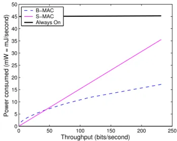
0 50 100 150 200 250
0 5 10 15 20 25 30 35 40 45 50
Throughput (bits/second)
Power consumed (mW = mJ/second)
B−MAC S−MAC Always On
Figure 8: The measured power consumption of maintaining a given throughput in a 10-node network. As the throughput increases, the overhead of S-MAC’s SYNC period causes the power consumption to increase linearly. The throughput is the average node bitrate (number of data bytes sent in a 10 second time period) in the 10 node network.
up and reprogrammed as quickly as possible. To find the channel utilization under congestion, we placednnodes equidistant from a receiver. Each node transmitted as quickly as possible with the MAC protocol providing collision avoidance. We increased the of-fered load by adding transmitters. There is no node or radio duty cycling in this test. The throughput achieved by B-MAC and S-MAC is shown in Figure 7.
In general, better throughput is attained with fewer nodes trying to saturate the channel. With one transmitter, B-MAC outperforms MAC broadcast mode (RTCTS disabled) by 2.5 times and S-MAC unicast mode (RTS-CTS enabled) by 4.5 times. B-S-MAC out-performs S-MAC for broadcast traffic due to more sophisticated CCA and lower preamble overhead. For unicast traffic, S-MAC suffers from the overhead of RTS-CTS exchanges. Instead of us-ing control messages like RTS-CTS for hidden terminal support, B-MAC’s relies on higher layer services to send data in accordance with their traffic pattern. These services implement the appropri-ate hidden terminal support for their workloads. For example, after sending a multihop message, all nodes in the cell should refrain from transmitting until one packet time has elapsed to allow the parent to retransmit up the tree as proven to be more efficient than control messages for multihop traffic in [20]. By allowing the ser-vice to decide, many costly control message exchanges are elimi-nated.
B-MAC exceeds the performance of S-MAC, but does not trade off fairness in the process. The test in Figure 7 uses a short ini-tial random backoff proven in [20] to provide fair channel utiliza-tion. By analyzing our dataset, we found that each node in the test achieves no more than 15% more bandwidth than any other node. To yield even higher throughput with B-MAC, we can discard fair-ness as a requirement. Each transmitter can set its backoff to zero and take control of the channel. As the number of nodes increases, channel contention and the capture effect3causes B-MAC’s perfor-3
The capture effect occurs when overlapping packets are sent due to one node sensing that the channel is clear while another node is in the process of switching to transmit mode [10, 14].
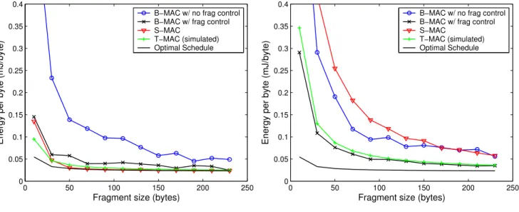
0 50 100 150 200 250 0
0.05 0.1 0.15 0.2 0.25 0.3 0.35 0.4
Fragment size (bytes)
Energy per byte (mJ/byte)
B−MAC w/ no frag control B−MAC w/ frag control S−MAC
T−MAC (simulated) Optimal Schedule
(a) 10 second message generation rate
0 50 100 150 200 250
0 0.05 0.1 0.15 0.2 0.25 0.3 0.35 0.4
Fragment size (bytes)
Energy per byte (mJ/byte)
B−MAC w/ no frag control B−MAC w/ frag control S−MAC
T−MAC (simulated) Optimal Schedule
(b) 100 second message generation rate
Figure 9: The effective energy consumption per byte at node C for a network as shown in Figure 10. Each node generates a message every 10 seconds (left) and every 100 seconds (right) consisting of 10 fragments of the size given on the x-axis.
mance to converge to S-MAC’s performance. Since S-MAC uses a longer preamble, a larger portion of the channel is dedicated to incoming signal synchronization by the receiver. Using B-MAC’s control interfaces, the preamble may be set to the same length as S-MAC or scale up as the channel contention increases.
To illustrate the effectiveness of a configurable MAC protocol for sensor networks, we implemented the RTS-CTS scheme described in Subsection 4.3. This scheme illustrates one method a service may employ to mitigate the hidden node problem and increase fair-ness with B-MAC. Since B-MAC can utilize 2.5 times more of the channel using the CCA algorithm from Section 3, the RTS-CTS implementation using B-MAC actually provides double the throughput of S-MAC. When many nodes compete for the channel, B-MAC with RTS-CTS support provides identical performance to S-MAC. This test illustrates that system services, like RTS-CTS, built using B-MAC’s interfaces does not hinder protocol perfor-mance.
6.2
Energy vs. Throughput
We designed B-MAC to run at both low and high data rates con-figured by services relying on it. Low duty cycle applications have extremely low network throughput; however some application ser-vices, such as bulk data transfer, stress the high throughput func-tionality of the MAC protocol. To evaluate how increased through-put affects power consumption, we vary the transmission rate of 10 nodes in a single cell. We bound the latency such that the data must arrive within 10 seconds. For B-MAC, the optimal check in-tervaltiis calculated for the traffic pattern, the test is run, and the energy consumption is calculated. For S-MAC, the optimal duty cycle is calculated for the traffic pattern such that the data arrives within the 10 second period. The results are shown in Figure 8.
At low data rates, S-MAC can use an extremely low duty cycle to transmit and receive the data. As the amount of data increases, so must S-MAC’s duty cycle. When the duty cycle increases, there are more active periods each with a dedicated SYNC period. Due to the overhead of the SYNC period at the beginning of each wakeup, the S-MAC energy consumption increases linearly. In B-MAC, at low
throughput we send long preambles with a long check intervalti. Because of the tradeoff between idle listening and packet length, the overhead dominates the energy consumption. The overhead of LPL is mitigated by a more frequent check interval when the throughput exceeds 45 bits per second. Note that B-MAC’s power consumption below 45 bits per second is within 25% of S-MAC’s power consumption; however, B-MAC has significantly less state and no synchronization requirements. Services using B-MAC may easily reconfigure the link protocol to change the check interval based on the network bandwidth whereas services using S-MAC must force it to create a new schedule and resynchronize.
6.3
Fragmentation
Small periodic data packets are the most common workload in sensor networks, but certain cases arise where larger transfers are needed. S-MAC supports large message fragmentation within the MAC protocol using an RTS-CTS exchange for channel reserva-tion. To compare B-MAC directly to S-MAC’s design goal of ef-ficient message fragmentation, we devised an experiment to match those done by the authors of S-MAC in [23]. Using the network configuration in Figure 10, we transmitted packets from sources A and B to sinks D and E by routing through C.
A
B
C
D E
Figure 10: X network configuration used for packet fragmen-tation tests.
As in [23], our test sent 10 fragments per message. We var-ied the fragment size and measured the energy consumed for that transfer. C is the energy bottleneck node in the test network–C will
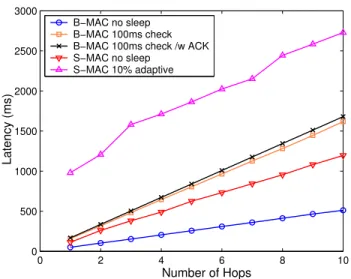
0 2 4 6 8 10 0
500 1000 1500 2000 2500 3000
Number of Hops
Latency (ms)
B−MAC no sleep B−MAC 100ms check B−MAC 100ms check /w ACK S−MAC no sleep
S−MAC 10% adaptive
Figure 11: The end-to-end latency is a linear function of the number of hops in the network. As the overhead of the MAC protocol increases, so does the slope of the latency.
cease operation before any other node since it must both receive and relay packets. We evaluate the energy required to deliver the fragments with S-MAC running at 10% duty cycle with adaptive listening. B-MAC is configured with the default parameters from Table 3. Figure 9(a) shows the energy cost per byte at node C when a message (consisting of 10 fragments) is sent every 10 seconds. Figure 9(b) show the energy cost per byte when the message gen-eration interval is once every 100 seconds.
B-MAC without fragmentation control is simply the B-MAC pro-tocol with the default parameters. Each fragment is an independent packet with a long preamble. But, the middleware service could adjust the MAC protocol to minimize the energy consumed during bulk transfer. In the measurements with fragmentation control, a message fragmentation service is built using B-MAC’s interfaces provided in Figure 1. The first fragment of the message is sent with LPL enabled and extra bytes to inform the receiver of the number of fragments. The remaining fragments are sent with LPL disabled. After the last fragment, the sender and receiver reenable LPL. With this flexibility, we achieve significant power savings and efficiency essentially identical to S-MAC without the additional overhead, in-cluding RAM and ROM usage. When the message transmission period is large (as in Figure 9(b)), the overhead of S-MAC is read-ily apparent; the energy consumption per byte of both S-MAC and T-MAC is greater at all fragment sizes than B-MAC with fragmen-tation support. The na¨ıve B-MAC approach with long preambles for each fragment yields the same power consumption as S-MAC without the additional complexity. When there is no activity on the channel, T-MAC removes the overhead incurred by S-MAC by using adaptive active periods to return to sleep much quicker. Fig-ure 9 shows that the energy cost of breaking up a short message into even shorter fragments is so high in all of our protocols that it is simply not a viable option in sensor networks.
6.4
Latency
The authors of S-MAC argue that when the MAC protocol is permitted to increase latency, S-MAC can reduce the node’s duty cycle and conserve energy. A test for evaluating end-to-end latency was devised in [23]. We have reproduced their tests to provide a direct comparison between B-MAC and S-MAC. The test is run
0 2 4 6 8 10
0 50 100 150 200 250 300 350 400 450 500 550
Latency (s)
Energy (mJ)
B−MAC S−MAC Always On
Figure 12: As the latency increases, the energy consumed by both B-MAC and S-MAC decreases. The point illustrated on the B-MAC line is the default configuration as shown in Table 3. The point on the S-MAC line is the default S-MAC configura-tion at 10% duty cycle with adaptive listening.
Source Sink
11 10 9 3 2 1
Figure 13: 10 hop configuration used for multihop end-to-end latency tests.
on a 10-hop network shown in Figure 13. In each test, the source node sends 20 messages with a payload of 100-bytes. There is no fragmentation on any message.
The latency at each hop of the network is measured with the method described in Section 5. S-MAC is tested at a 10% duty cycle with adaptive listening. B-MAC is tested with the default parameters. The results are shown in Figure 11. We are able to reproduce the latency data from [23] and it fits the previously pub-lished results.
The latency of B-MAC and S-MAC increase linearly. When duty cycling is disabled, the effect of RTS-CTS exchanges in S-MAC result in a much steeper slope than B-MAC. For low power com-munications, B-MAC has a slope almost identical to S-MAC with adaptive listening, however the y-intercept is much lower. Since the first packet cannot be sent until an S-MAC active period, it is delayed by at most 1150 milliseconds. Through adaptive listening, S-MAC does not incur an expected 1150 milliseconds additional delay at each hop. One protocol feature of B-MAC, link layer ac-knowledgments, increases latency by an insignificant amount.
To better evaluate the effect of increasing the latency to reduce power consumption, we fixed the throughput to one 100 byte packet per 10 second interval. We measured the end-to-end latency of the 10 hop network and varied the duty cycle of S-MAC. We also chose the optimaltifor B-MAC given the latency and throughput. The results are shown in Figure 12.
For latencies under 6 seconds, B-MAC performs significantly better than S-MAC. As S-MAC approaches the 10 second latency limit, its power dips below B-MAC. When the latency exceeds 3 seconds, B-MAC’s power consumption is bounded by the cost of idle listening. In contrast, the best case performance of S-MAC
0 0.5 1 1.5 2 2.5 3 3.5 x 10⁴ 0
0.5 1 1.5 2 2.5 3
Number of packets forwarded or sent
D
ut
y
C
yc
le
(%
)
1 hop from base station
Leaf nodes
Figure 14: As the traffic around a node increases, so does the duty cycle when using the B-MAC protocol with LPL. The node one-hop from the base station forwards 85% of the packets in the deployment yet achieves a lower duty cycle by minimizing the preamble length for packets sent to the base station.
shown in Figure 12 relies on S-MAC synchronizing the entire 10-hop network and using adaptive listening to transmit the data through the network in one active period. Figure 12 shows the importance of reconfiguration in wireless sensor networks. If the application’s required latency is relaxed, S-MAC could achieve lower energy consumption than B-MAC; however S-MAC operates at a single setting, is not reconfigurable, and thus cannot realize these energy savings.
7.
MACROBENCHMARK ANALYSIS
The application model in Section 4 predicts the performance of a monitoring application for wireless sensor networks using the B-MAC protocol. In this section, we examine the behavior of a real-world monitoring application called Surge. We examine Surge’s duty cycle and compare the results to predictions from the ana-lytical model. The empirical characterizations from Section 6 are evaluated with the networking results from Surge. We also examine the use of B-MAC’s interfaces for simple optimizations that have a large impact on the network’s lifetime.
Surge is a periodic data collection application that acquires sam-ples from the node’s sensors, sends the readings, and sleeps. It was deployed by placing 14 nodes throughout a 30 meter by 20 me-ter home. The nodes automatically configured themselves into an ad-hoc routing network. Surge collects data from each node once every three minutes. Instead of collecting sensor data, we acquired statistical information from B-MAC about its performance (see Sec-tion 5 for the energy indicators implemented in B-MAC). Each node transmits its energy usage, battery voltage, estimated link quality to surrounding nodes, and its current parent. Data from Surge is used to verify that the network performance matches the microbenchmarks from Section 6.
Using our estimate of lifetime versus check interval for a given sample period (see Figure 6), we selected a 100ms check
inter-valti. By evaluating the node communication range and overall
size of the network, we expected a maximum neighborhood size of 5 nodes. To be conservative, we calculated the preamble length
0 1 2 3 4 5
0 0.5 1 1.5 2 2.5 3
Number of hops
Duty Cycle (%)
Average Duty Cycle Logarithmic Fit
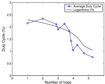
Figure 15: The position in the network dictates the amount of traffic flowing through that level. As we approach the base sta-tion, nodes handle an increasing number of packets. The av-erage duty cycle is computed by finding the avav-erage for nodes at a given hopcount. Fractional hopcounts are correlated with nodes that oscillated between two levels of the network. Note that nodes one-hop away from the base station can achieve a lower duty cycle because the base station is always on. By re-configuring B-MAC to use short packets, nodes one-hop from the base station survive up to 50% longer.
and check interval with a neighborhood size of 10. Using a larger neighborhood may cause us to overshoot the optimal configuration, but Section 4 and Figure 5 show that using a longer check interval is less detrimental to the overall lifetime than checking the channel too often.
Since the most important thing in a monitoring network is re-liably reporting the data, we must confirm that B-MAC success-fully supports multihop data reporting. Our implementation uses the default multihop routing protocol from the TinyOS distribution, called MintRoute. After integrating B-MAC with MintRoute, the routing layer enables B-MAC’s link layer acknowledgments. Upon a failed acknowledgment, MintRoute retransmits the message up to five times. The Surge application was run for a period of 8 days. We collected over 40,000 data packets profiling the performance of a real world wireless sensor network.
During the Surge deployment, the network yielded over 98.5% packet delivery while some nodes achieved an astounding 100% success rate. In our deployment, there were a total of 71 times where a node decided to change its parent–and consequently changed the routing tree–as a result of environmental changes altering the communication topology. In confirmation of Woo and Zhao’s iden-tification of gray areas, high-quality links that were stable for hours were intermittently broken due to environmental changes.
The base station was placed at a convenient location to install in-frastructure in a corner of the network. From the data collected by the Surge application, we can determine the actual duty cycle of our deployed network. Surge reports the values of our instrumented op-eration counters. These counters translate into a duty cycle based on a 12mA constant current consumption while active. From the duty cycle, we can extrapolate the network lifetime. Figure 14 shows the measured duty cycles of each node in the network. The worst case duty cycle of 2.35% indicates that the first node should
0 1 2 3 4 5 6 0
100 200 300 400 500 600 700 800 900 1000 1100
Number of hops
Latency (ms)
B−MAC Avg Latency Std Dev B−MAC Avg Latency B−MAC Min Expected Latency
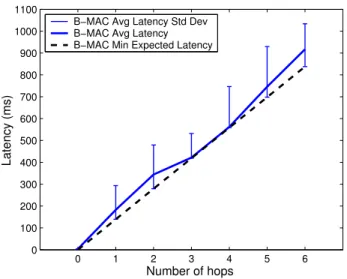
Figure 16: The average latency of packets being delivered by the Surge application is dependent on the traffic in the network and reliability of each link. The average exceeds the expected latency because retransmissions add additional latency to each packet.
exhaust its battery supply approximately 369 days (1.01 years) into the deployment.
Our data shows that each node has an average of 5 neighbors, less than our maximum estimate of 10. Additionally, some nodes on the edge of the network have less than a 1% duty cycle. We attribute the lower duty cycle to the significant reduction in traffic at the edges of the network as compared to central nodes routing a large amount of data. The variance in leaf node duty cycle is due to differences in local neighborhood size.
Although the network is homogeneous, we can exploit that the base station runs with a different duty cycle (since it is always on) than the data collection network. Instead of sending packets with long preambles, nodes one hop away send packets with only an 8 byte preamble to the base station. Figure 14 shows the node duty cycle versus number of packets routed through the node. There was one node that despite forwarding almost 35,000 packets (about 85% of all data packets), had a duty cycle equal to nodes forward-ing less than 10,000 packets. This node was critical to reliable data delivery–by forwarding most of the packets, it would have ex-hausted its battery supply first and caused a network partition. Fig-ure 15 shows the duty cycle vs. multihop level in the routing tree. The node routing 35,000 packets one hop from the base station was able to alter its MAC behavior (send short preambles) based on its position in the network and optimize performance.
To validate our model, we calculated the expected lifetime based on the parameters of our deployment. For the functionchildren(i) in our model, we performed two calculations: the first assumes that the routing algorithm produces a balanced binary tree, the sec-ond assumes the worst case routing tree–a line topology where all traffic must be forwarded by the node one hop from the base sta-tion. With a balanced tree and no routing protocol reconfigura-tion of B-MAC, the first node should exhaust its battery supply in 385 days (1.06 years). For a line, the worst case lifetime is 256 days (0.71 years).
In the presence of the one-hop optimization and a balanced tree, we expect that nodes one-hop from the base station will exhaust their battery supply 549 days (1.49 years) into the deployment,
nodes two-hops exhaust their supply in 542 days (1.48 years). For a line, the expected lifetime of the node one hop from the base station is 391 days (1.07 years). Unfortunately the nodes in our deployment did not form a balanced tree, nor did they form a line. Our measured power consumption data shows that a node one hop away will survive for 1.13 years, slightly higher than our 1.07 year estimate for a line. At two hops in the Surge application, the worst case lifetime of 1.01 years is directly between our estimates of 1.48 years for a balanced tree and 0.71 years for a line. This data validates the model; however, protocol designers must care-fully build network services that uniformly distribute routing (and thereby uniformly distribute energy consumption) throughout the network.
Without the one-hop to base station optimization, worst case power consumption is up to 50% higher. The powered base station is a simple example of network heterogeneity; one could imagine much more heterogeneity with a hierarchy of devices. The dif-ferences between devices dictate other optimizations that may be implemented through bidirectional communication with the MAC protocol.
In addition to predicting the power consumption of the network, our empirical model also predicts the network latency that is intro-duced by the B-MAC protocol illustrated in Figure 11. Since Surge is a periodic application, message latency was measured by evalu-ating the variations in packet delivery rates. The latencies measured in our Surge deployment along with the predicted values are plotted in Figure 16. The average latency is slightly higher than the predic-tion. However the minimum latency for each network level exactly matches the predicted value. The difference between the average and minimum latencies is due to unexpected network congestion and packet loss. Surge retransmits messages to increase reliability when B-MAC indicates an acknowledgment failed. Upon retrans-mission, the message incurs additional latency.
8.
DISCUSSION
Our benchmarks have shown that a small amount of information from services using B-MAC can provide significant power savings. Additional power savings can be achieved through more informa-tion about the applicainforma-tion and its operainforma-tion. In this secinforma-tion, we discuss the implications and other uses of these ideas.
Because B-MAC is lightweight and configurable, many sensor network protocols may be implemented efficiently using its prim-itives. S-MAC and T-MAC may be implemented as services that use B-MAC as the underlying link protocol. S-MAC and T-MAC are more than just link protocols; they perform synchronization, or-ganization, fragmentation, and hidden terminal support and could benefit from B-MAC’s flexibility. These protocols could be built on B-MAC in a modular way to allow applications and other services to use only necessary subsets of the mechanisms they provide.
To mitigate the cost of reception incurred with B-MAC with LPL, a packet could be sent cyclically with a short preamble. Al-though this does not reduce the transmission cost, it reduces the time of receiving a packet to:
trx≤2×(Lpreamble+Lpacket)×trxb
Note thatLpreambleis reduced from the long LPL preamble to only 8bytes. The node can return to sleep for the check interval after receiving a packet or can perform early rejection much quicker than packets sent with the long preambles.
We showed in Section 7 that using the node’s level in the tree can assist in reducing the duty cycle. To reduce transmission en-ergy consumption, each node may learn the offset of the check in-tervaltithat their parent wakes up to sample the channel. Knowing