Vol. 7, No. 3, 2014, 289-303
ISSN 1307-5543 – www.ejpam.com
Robust Control System for Spacecraft Motion Trajectory
Zarina Samigulina
1,∗, Olga Shiryayeva
2, Galina Samigulina
2, Hassen Fourati
31Department “Automation and control”, Kazakh National Technical University after K.I.Satpayev,
Almaty, Kazakhstan
2Laboratory “Intellectual control systems and networks”, Institute of Informatics and Control
Prob-lems, Almaty, Kazakhstan
3 Networked Controlled System Team (NeCS), Automation and Control Department, University
Joseph Fourier, Cedex, France
Abstract. In aerospace field the economic realization of a spacecraft is one of the main objectives which should be accomplished by conceiving the optimal propulsion system and best control programs. This article focuses on the implementation of uncertain control system theory and development of a robust control system of Spacecraft Motion Trajectory (SMT). The proposed strategy involves the nonlinear mathematical model of SMT expressed in the central field, which is linearized by the Taylor expansion, and model reference Adaptive Control Approach (ACA) with the second Lyapunov method to offer a high rate and unfailing performance in the functioning. The efficiencies of the linearization procedure and the control approach are theoretically investigated through some realistic simulations and tests under MATLAB.
2010 Mathematics Subject Classifications: 62F35
Key Words and Phrases: Robust control system, Spacecraft Motion Trajectory, adaptive control ap-proach, nonlinear system modeling, reference model, Lyapunov method
1. Introduction
Most modern controlled processes are complex, multi-dimensional nonlinear systems and have as a potential application the conception of flying objects for the aerospace industry[18]. Sometimes, for these objects the first problem is related to the development of a mathematical model because there is a little information about the data that describe the object behavior or there is usually a change in the structure and/or parameters of the mathematical model during the spacecraft missions. The second problem is related to the control functions.
∗Corresponding author.
Email addresses:[email protected](Z. Samigulina),[email protected](O. Shiryayeva), [email protected](G. Samigulina),[email protected](H. Fourati)
In literature, the adaptive control approaches has been widely developed in aerospace ap-plications on the base of a large panel of methods. The authors developed in[16] a method based on the self-learning to accomplish a precise mission of the spacecrafts. The developed adaptive controllers through these methods used the principles of characteristics frequency stabilization and the reference model. In[10], an attitude adaptive control of satellites in el-liptic orbits is proposed. The paper presents a novel non certainty-equivalent adaptive control system for the satellites pitch control. The adaptive law is based on the attractive manifold design using filtered signals for the synthesis. The developed work in [11] is devoted to the adaptive control of a flexible spacecraft in noisy environment. A new control law for a large angle rotational maneuver of the spacecraft is derived. The control system includes a state predictor to generate the estimates of the unknown parameters to be used in the feedback law. The controller is synthesized using only the pitch angle and its first derivative. A new design of a simple adaptive system for the rotational maneuver and the vibration suppression of an orbiting spacecraft with flexible appendages is proposed in[14]. The control output variable is chosen as the linear combination of the pitch angle and rate. A simple adaptive control law is derived for the pitch angle control and the elastic mode stabilization. The adaptation rule requires only four adjustable parameters and the structure of the control system does not de-pend on the order of the truncated spacecraft model. The authors in[21]described a hybrid control scheme for a flexible spacecraft. To obtain good static and dynamic characteristics, the hybrid control scheme is put forward with a variable structure and an intelligent adaptive control method.
adaptive output feedback tracking control of multiple spacecrafts is presented. The control law is designed to provide a filtered velocity measurement and a desired adaptive compensation with a semi-global and asymptotic position tracking. The proposed control law is simulated in the case of two and three spacecrafts and the results showed the semi-global and asymptotic tracking of the relative position errors.
Demand for high performance in systems with nonlinear behavior and model uncertainties is one of most challenging area in control theory[2]. An adaptive robust controller represents a systematic way to design a controller for such requirement, and it combines adaptive and robust control approaches to preserve the advantages of the both methods while overcoming their drawbacks. In literature for spacecraft the approach that has been developed in [9] was implied to combine the adaptive robust controller with dynamic backstepping method. In this method the robust controller is used as the main controller for trajectory tracking, and adaptive controller tries to decrease the uncertainty and helps to reduce tracking error especially at steady state.
In this article we developed an adaptive control strategy for robust control system of SMT. This approach involves the reference model which includes the information on the desired dynamics of the spacecraft trajectory. Robustness in SMT model is determined by the uncertain parameters.
We chose the control law which is necessary to describe the purpose of control and we selected tunable parameters of the mathematical model and the purpose of adaptation. After that, we selected the adaptation algorithm based on the gradient type. The algorithm uses the error between the output of the considered dynamic system including the reactive acceleration and the reference model. Finally, we synthesized the adaptive controller taking into account the random disturbances. As a result, we obtained the system which works as follows: the spacecraft is moving according to the desired optimal trajectory, in the case of deviations from the desired trajectory it triggers the adaptive controller which returns the system to the original optimal trajectory.
The primary contributions of this paper can be stated within the following points:
1) The linearization of the mathematical model of SMT, which is proposed in [7]. The lin-earization of this nonlinear time-varying model is achieved by a Taylor expansion, which allows to obtain a satisfactory linear time-invariant reference model to be used in the adap-tive control.
2) The design of an adaptive control system of SMT based on the proposed linearized reference model and the Lyapunov theory. In our knowledge, the use of adaptive control within the SMT model is new and leads to obtain a satisfactory control of the spacecraft trajectory.
2. Robust Mathematical Model of SMT
In this section, the mathematical model of robust control system of SMT is firstly presented [7]and secondly linearized to be used later in the development of the adaptive control strategy. In this paper, the mathematical model of SMT in a central field is considered. The model is built for the initial elliptical orbit and expresses a transition from an elliptical to parabolic orbit (for example) in the interplanetary flight and is obtained by using the Pontryagin Maximum Principle[7].
2.1. Optimal Mathematical Model of SMT
Let consider the mathematical model of SMT which is described by the nonlinear differen-tial equations system based on the boundary conditions[7]:
˙
p(t) =2 p(t)(3/2)(Q(t) +1)−1aφ
˙
Q(t) = −p(t)(−3/2)(Q(t) +1)2L(t) +2pp(t)aφ ˙L(t) = p(t)(−3/2)
(Q(t) +1)2Q(t) +pp(t) (Q(t) +1)−1L(t)aφ+
p
p(t)ar
(1)
where p(t) ∈ ℜ denotes the parameter of the osculating ellipse and {Q(t), L(t)} ∈ ℜ de-note the phase coordinates. The accelerationsar, aϕ ∈I(ℜ)define the components of the reactive acceleration in the spherical coordinates andu(t)is the command signal and robust character of the system:
ar=ar±∆ar, aϕ=aϕ±∆aϕ,
ar, aϕ ∈I(ℜ),ar, aϕ∈ ℜ
where I(ℜ)- set of uncertain interval parameters with real bounders,∆ar ∆aϕ - parameter deviations from nominal values due to external perturbations.
The initial conditionsp0,Q0,L0 that determine the optimal trajectory can be written in terms of the initial conditions of the eccentricityǫ0 and true anomalyν0such as:
p0=1−ǫ02; Q0=ǫ0cosν0; L0=ǫ0sinν0 (2)
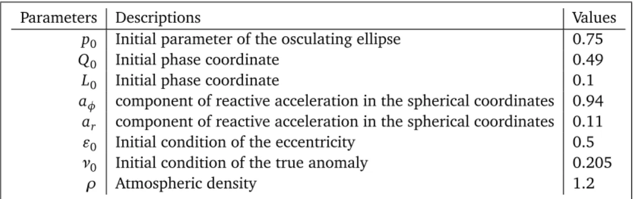
For more clarity, the Table I summarizes the main parameters of SMT mathematical model (1).
2.2. Linearization of the SMT Mathematical Model
The mathematical model of SMT is described by the nonlinear differential equations system (1). The first step to design an ACA for the spacecraft model states is the linearization of the system (1) using the Taylor series expansion, as detailed in[6, 17].
To work with the uncertain system with interval-set parameters the results were obtained by the authors according to which the uncertain parameters can be the key point with the use of auxiliary parameters[4]:
and definingqkey parametersdq∈ ℜinterval valued∈I(ℜ), as:
dq∈d,
dq=
(
dq, z=1
dq, z=−1
In accordance with this method there can be used uncertain parametersar, aϕ ∈I(ℜ) as the point parameters with valuesaϕ=0.94,ar=0.11.
The mathematical model can be expanded in a Taylor series around the operating point. Since the deviations from the operating point are small, the expansion takes only the term with the degree 1. The resulting equations after expansion are subtracted from the equilibrium equations which lead to obtain a linearized equations around the operating point.
Let consider the first equation of the system (1):
˙
p(t) =2 p(t)(3/2)(Q(t) +1)−1aφ (3) The equation (3) can be re-written in the following way:
˙
p(t)−2 p(t)
(3/2)
·aφ
Q(t) +1 =0 (4)
The equation (4) can be defined as a functionF ˙p,p,Q,t:
F ˙p,p,Q,t=˙p(t)−2 p(t)
(3/2)
·aφ
Q(t) +1 =0 (5)
To linearize the equation (3), the functionF ˙p,p,Q,tis decomposed in Taylor series around of the operating point 0,p0,Q0
, where p0=0.75 andQ0=0.49 (see Table I).
Table 1: SMT model paramters
Parameters Descriptions Values
p0 Initial parameter of the osculating ellipse 0.75
Q0 Initial phase coordinate 0.49
L0 Initial phase coordinate 0.1
aφ component of reactive acceleration in the spherical coordinates 0.94
ar component of reactive acceleration in the spherical coordinates 0.11
ǫ0 Initial condition of the eccentricity 0.5
ν0 Initial condition of the true anomaly 0.205
ρ Atmospheric density 1.2
Then, the exclusion of the terms of the second and higher orders in this expansion leads to the following equation:
F ˙p,p,Q,t=F0+∂F
∂˙p∆˙p(t) +
∂F
∂p∆p(t) +
∂F
By using the equation (6) and the parameteraφ=0.94 (see Table I), it is possible to find the value of the functionF0 and the partial derivative terms ∂∂F˙p, ∂∂Fp and ∂∂QF:
F0=0 ∂F
∂˙p
0=1 ∂F
∂p
0=− 3 2·
2p(03/2)−1·aφ
Q0+1 =−1.63
∂F ∂Q 0=
2p(03/2)·aφ
(1+Q0)
2 =0.53
(7)
Then, equation (6) can be written in deviations from the operating point 0,p0,Q0
:
∆˙p(t) =1.63∆p(t)−0.53∆Q(t) (8)
The equation (8) represents the linearized form of the first nonlinear equation (3) of the math-ematical model (1). In the same way, we applied the linearization method to the second and third motion equations of SMT model (1).
Finally, we obtained the following linear mathematical modelP′of the nonlinear system (1):
∆˙p(t) =1.63∆p(t)−0.53∆Q(t)
∆Q˙(t) =−0.46∆Q(t)−3.42∆L(t) +1.37∆p(t)
∆˙L(t) =0.55∆L(t) +5.63∆Q(t)−2.13∆p(t)
(9)
The linearized mathematical model P′ of SMT will be used below in the design of the adaptive control method.
3. Adaptive Control Approach Design for SMT Model
3.1. General Overview of the ACA Block Diagram
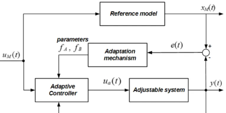
the controlled plant y(t)are different from the reference values xM(t), then the error sig-nal e(t) = xM(t)− y(t) is provided as an input to the adaptation law, which contains the adaptation algorithm. In this paper, the adaptation is developed using the Lyapunov theory.
Figure 1: Block diagram of the model reference adaptive control of SMT
When the spacecraft deviates from its trajectory, the ACA acts on the spacecraft control system to correct this deviation and follow the optimal reference trajectory. In other words, when the states of the adjustable system y(t)are different from the reference values xM(t), then the error signale(t)is provided as an input to the adaptation law block, which contains the adaptation algorithm based Lyapunov theory.
3.2. Model-Reference Adaptive Control Algorithm Design
The linearized model of SMT (9) can be written in the following matrix representation:
∆˙p(t) =1.63∆p(t)−0.53∆Q(t) +b1u(t)
∆Q˙(t) =−0.46∆Q(t)−3.42∆L(t) +1.37∆p(t) +b2u(t)
∆˙L(t) =0.55∆L(t) +5.63∆Q(t)−2.13∆p(t) +b3u(t)
(10)
Around the equilibrium point, we consider x1(t) = ∆p(t) ≈ p(t), x2(t) = ∆Q(t)≈Q(t),
x3(t) = ∆L(t)≈ L(t)as the state variables of the mathematical model (10), then we can
re-write the linear system such as:
∆˙p(t)
∆Q˙(t)
∆˙L(t)
=
1.63 −0.53 0 1.37 −0.46 −3.42
−2.13 5.63 0.55
∆p(t)
∆Q(t)
∆L(t)
+
1 0 0 0 1 0 0 0 1
u(t) (11)
Then, the mathematical model (11) can be written as a general state-space representation of a linear system:
˙
x(t) =Ax(t) +Bu(t) (12)
matrix representing the linearized effects of the control parameters andu(t)is the control law vector.
The adjustable system of SMT shown in Figure 1 can be written according to the form of the linear system (12) but due to the changing of the system (1) proprieties and the operating point, its matrices Aand B are poorly known and their values are time-dependent. These drawbacks can be addressed by the application of a model reference adaptive control law[12] that results in a time-dependent feedback control matrix f(t). Therefore, we consider in the upper portion of the diagram in Fig. 1 the reference model that represents the desired closed-loop dynamics of the system. This reference model should correspond to the optimal trajectory model of SMT (11) and is established by the selection of its fundamental matricesAM andBM:
˙
xM(t) =AMxM(t) +BMu(t) (13)
where xM(t) = pM(t)QM(t)LM(t)T is the state vector of the reference model and the fundamental matricesAMandBMare equal to the state matrixAand the input matrixBof the
mathematical model (11), which leads to obtain:
AM =
1.63 −0.53 0 1.37 −0.46 −3.42
−2.13 5.63 0.55
, BM=
1 0 0 0 1 0 0 0 1
(14)
The lower portion of the diagram in Fig. 1 represents the mathematical model of the adjustable system which is given by the following state-space representation:
˙
y(t) =AS(e,t)y(t) +BS(e,t)ua(t) (15)
where y(t) =ps(t)Qs(t)Ls(t)
T
is the state vector of the adjustable system,
AS(e,t)∈ ℜ3×3 and BS(e,t) ∈ ℜ3×3 are time-varying matrices whose terms depend on the state generalized error vector e1(t) e2(t) e3(t)
T
and
ua(t) = fy(t)· y(t) +fM(t)·uM(t)
is the control law wherefy(t)andfM(t)represent two state variable feedback control matrices which will be tuned later based on the second method of Lyapunov[1].
For tuning of fy(t),fM(t)the input signal of the adjustable system (15) isuM(t). The error
vectore(t)in the middle portion of the diagram is calculated as the discrepancy between the states of the reference model and the active response of the adjustable system with input signal
uM(t):
e(t) =xM(t)−y(t) (16)
The error vectore(t)becomes as an input information to the adaptation block where an adap-tation law is implemented by using the Lyapunov theory[1], resulting in an asymptotic adapta-tion where the three states control errors will converge to zero regardless of initial condiadapta-tions. Firstly, we differentiate the state generalized error vector in (16) to obtain its derivative:
After, we define a Lyapunov functionV, which includes the generalized errore(t). The chosen function takes the following form[1]:
V =eT(t)·P·e(t)
+t r¦AM−AS(e,t)
T
·fA−1·AM−AS(e,t)
©
+t r¦BM−BS(e,t)T ·fB−1·BM−BS(e,t)©
(18)
According to the considered Lyapunov function, V, and the second Lyapunov method, the matrix P should be positive definite and skew-symmetric, P = PT > 0, and fA and fB are positive parameters of the adaptive mechanism, which will be defined later.
When differentiating (18), the derivative of the Lyapunov function can be written such as:
˙
V =eT(t) ATM·P+P·Ae(t)
+2t r{[AM−AS(e,t)]T. . .[P·e(t)· yT(t)−fA−1·A˙S(e,t)]}
+2t r{[BM−BS(e,t)]T(P·e(t)·uT(t)−fB−1·B˙S(e,t)]}
(19)
The first term in (19) is negative definite for all e(t)6=0 and the second and third terms are identically equal to zero if one chooses the following adaptation laws[12]:
˙
AS(e,t) = fA·(P·e(t))· yT(t) (20)
˙
BS(e,t) = fB·(P·e(t))·u(t) (21)
When integrating (20) and (21), one obtains:
AS(e,t) =
Z t
0
fA·(P·e(t))·yT(t)dτ+AS(0) (22)
BS(e,t) =
Z t
0
fB·(P·e(t))·u(t)dτ+BS(0) (23)
One notes that fA and fB are used to establish a functional relationship between AS(e,t),
BS(e,t) and the values of the error vector e(t) in the interval 0 ≤ τ ≤ t [12]. Then, the
problem of model reference adaptive control system can be seen as a regulation problem for the spacecraft system displaced from its equilibrium state (defined by AM = AS, BM = BS) using the adjusted parameters fAand fB(see Figure 1). Therefore the adaptive control design
problem can be specified from the following proposition:
Proposition 1. Given an unknown initial differencesAM−AS(t),BM−BS(t)between the parameters of the reference model and those of the adjustable system at t=t0and a known initial state generalized error vector e t0
=x t0
−y t0
, find an adaptation law independent of the initial conditions which achieves an asymptotic adaptation characterized by:
lim
t→∞e(t) =0 (24)
lim
t→∞AS(t) =AM (25)
lim
Finally, the control lawua(t)for the adjustable system is established using the conditions (24)-(26) and the adjusted parameters fAand fB as follows[12]:
ua(t) =fy(t)· y(t) +fM(t)·uM(t)
d
d tfy(t) =fA·B T
S ·P·e(t)· y(t)
T
d
d tfM(t) =fB·B T
S ·P·e(t)·uM(t)
(27)
4. Simulation Results
This section aims to illustrate the performance and accuracy of the designed model refer-ence ACA via some numerical simulations carried out under MATLAB. The performed simula-tions concerned the linearization of SMT model and the adaptive control system design.
4.1. Simulation Results of SMT Model Linearization
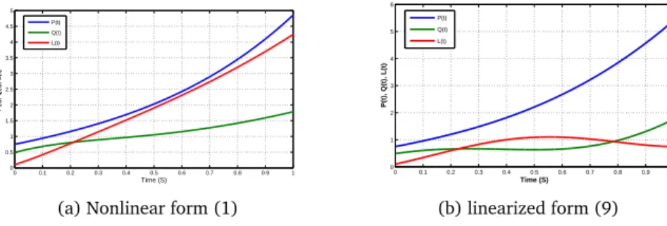
We carried out some realistic simulations of the states evolution of the SMT nonlinear math-ematical model (1) and its linearized version (9). The obtained results in Figures 2 (a) and (b) show the evolution of the osculating ellipsep(t)and the phase coordinates{Q(t),L(t)}
before and after linearization, respectively. The initial conditions presented in Table I. In accordance with Figure 2, the dynamics of the linearized mathematical model (Fig-ure 2b) corresponds to the dynamics of the nonlinear mathematical model (Fig(Fig-ure 2a), then we can used the linearized mathematical model (9) for solving the problem of the adaptive control synthesis.
0 0.1 0.2 0.3 0.4 0.5 0.6 0.7 0.8 0.9 1 0
0.5 1 1.5 2 2.5 3 3.5 4 4.5 5
Time (S)
P(t), Q(t), L(t)
P(t) Q(t) L(t)
(a) Nonlinear form (1)
0 0.1 0.2 0.3 0.4 0.5 0.6 0.7 0.8 0.9 1 0
1 2 3 4 5 6
Time (S)
P(t), Q(t), L(t)
P(t) Q(t) L(t)
(b) linearized form (9)
Figure 2: States evolution of the SMT model
4.2. Adaptive Control Algorithm Implementation under MATLAB
Algorithm 1. The adaptation algorithm steps implementation under MATLAB (tuning of the parameters fA, fB)
1) Take the initial conditions and parameters of the SMT mathematical model (see Table I).
2) Selection of the parameters fA, fB.
3) Calculation of the values of output signal of the reference model (13).
4) Calculation of the values of output signal of the adjustable system (15) with input signal
uM(t).
5) Calculation of the elements of the state generalized error vectore(t)by using (16).
6) Calculate the elements of the matrix ˙AS(t)and ˙BS(t)from (20) and (21).
7) Plot the results of the adjustable system and the reference model.
4.3. Simulation Results of the Adaptation Algorithm
The SMT linearized reference model and adjustable system are simulated based on the equations (13), (15), (16), (20), (21) and algorithm 1. Matrices of reference model and adjustable system, AM, BM, AS(t), BS(t), are selected in accordance with matrices AM, BM
(14). But the initial conditions of the adjustable system and the reference model are chosen different such as:
y1(0) y2(0) y3(0)
T
= pS(0) QS(0) LS(0)
T
= 0.1 0.2 0.01 T
xM1(0) xM2(0) xM3(0)
T
= pM(0) QM(0) LM(0)
T
= 0.75 0.489 0.102 T
Input signal for reference model is chosen asuM(t) =1, matrixP- unit matrix (positive definite and skew-symmetric). The implementation of the adaptation algorithm 1 were obtained the parameters for adaptive controller fA=1000, fB=1000.
0 0.1 0.2 0.3 0.4 0.5 0.6 0.7 0.8 0.9 1
0 1 2 3 4 5 6
Time (S)
Xm(t), Y(t)
Pm(t) Ps(t) Qm(t) Qs(t) Lm(t) Ls(t)
0 0.05 0.1 0.15 0.2 0.25 0.3 0.35 0.4 0.45 0.5 0 0.5 1 1.5 2 2.5 3 Time (S) Xm(t), Y(t) Pm(t) Ps(t) Qm(t) Qs(t) Lm(t) Ls(t)
Figure 4: Zoom on the states evolution of the adjustable system (15)
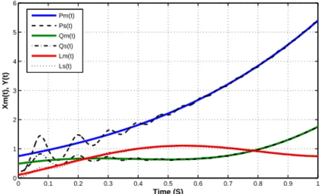
The obtained states evolution of the adjustable system (15) and the reference model (13) are compared for 1 second in Figure 3. This figure shows the states pS(t),QS(t),LS(t)of
the adaptive SMT scheme adapting itself with the reference pM(t),QM(t),LM(t). The first
interval, 0 to 0.5 seconds, of Figure 3 shows the adapted statespS(t),QS(t),LS(t)oscillate and adjust to converge to the desired states pM(t),QM(t),LM(t). The second interval, 0.5 to 1 sec, shows convergence settling smoothly to the desired reference. The obtained results prove that the adapted states of the SMT model can match with the desired reference model with the aid of the Lyapunov stability criterion which is applied in feedback for tuning the parameters to make the error between the reference and the plant tends to zero. For more clarity of the convergence rate, we took a zoom in Figure 4 of the first interval of the states evolution in Figure 3.
The generalized error vector of controle(t) = e1(t) e2(t) e3(t) T between the ref-erence model and the adjustable dynamic model of SMT is calculated from the equation (15) and is presented in Figure 5. It is clear that these errors converge to zero which proves the efficiency of the proposed adaptation algorithm.
0 0.2 0.4 0.6 0.8 1
−0.8 −0.6 −0.4 −0.2 0 0.2 0.4 0.6 Time (S) e1(t)
0 0.2 0.4 0.6 0.8 1
−0.4 −0.3 −0.2 −0.1 0 0.1 0.2 0.3 Time (S) e2(t)
0 0.2 0.4 0.6 0.8 1
−0.1 −0.08 −0.06 −0.04 −0.02 0 0.02 0.04 0.06 0.08 0.1 Time (S) e3(t)
e1(t) e2(t) e3(t)
Figure 5: The generalized error vector of controle(t)
4.4. The Adaptive Control Algorithm
Algorithm 2. The adaptive control algorithm
1) Take the initial conditions and parameters of the SMT mathematical model (see Table I).
2) Calculation of the values of output signal of the reference model (13).
3) Calculation of the values of output signal of the adjustable system (15) with adaptive con-trol law (27), where fA, fBare the parameters from algorithm.
4) Plot the results of the adjustable system (15) with adaptive control (27) and the reference model (13).
4.5. Simulation Results of the Adaptive Control Algorithm
The proposed ACA for the SMT linearized model is simulated based on the algorithm 2 (Figure 6). The matrices and initial conditions of the adjustable system and the reference model are chosen according to algorithm 1.
Figure 6: States evolution of the adjustable system (15) using the adaptive control (27) and the reference model (13)
Results of modeling (Figure 6) are identical to the results presented in Figure 3.
5. Conclusion
controller which returns the system to the original optimal trajectory. The obtained simulation results of the adaptive control strategy prove the efficiency and performance of the proposed adaptive control algorithm. The state errors of control converge to zero over a short period of 0.5 seconds.
ACKNOWLEDGEMENTS The authors are grateful to Professor Ioan Dore Landau (Gipsa -Lab, Grenoble, France) for constructive advice for improving this article.
References
[1] B R Andrievsky and A L Fradkov. Selected chapters of the control theory with the exam-ples on the language matlab. pages 308–310. Science, 2000.
[2] M Ataollahi and H D Taghirad. Adaptive robust controller design for non-minimum phase systems. The proceedings of TOK’11, Izmir, Turkey, 2011.
[3] J Bae and Y Kim. Adaptive controller design for spacecraft formation flying using sliding mode controller and neural networks. Journal of the Franklin Institute, 349(2):578–603, 2012.
[4] N A Bobylev. About positive definiteness of interval families of symmetric matrices. Au-tomation and Remote Control, 61(8):4–9, 2000.
[5] G Cruz, M D A Amato, and S D Bernstein. Retrospective cost adaptive control of spacecraft attitude. AIAA Guidance, Navigation, and Control Conference, 2012.
[6] F Golnaraghi, C Benjamin, and C B Kuo. Automatic Control Systems. 9th, Willey, 2009.
[7] G L Grodzovskii, N Ivanov, and V V Tokarev. Mechanics of space flight (optimization problem). Science, Moscow, 1975.
[8] A Jasim, V T Coppola, and S D Bernstein. Adaptive asymptotic tracking of spacecraft attitude. Journal of Guidance, Control, and Dynamics, 21(5):684–691, 1998.
[9] Y Jiang, Q Hu, and G Ma. Adaptive backstepping fault-tolerant control for flexible spacecraft with unknown bounded disturbances and actuator failures. ISA Transactions, 49(1):57–69, 2010.
[10] W L Keum and N S Sahjendra. Attractive manifold–based adaptive solar attitude control of satellites in elliptic orbits. Acta Astronautica, 68(1-2):185–196, 2011.
[11] W L Keum and N S Sahjendra. L adaptive control of flexible spacecraft despite distur-bances. Acta Astronautica, 80(11):24–35, 2012.
[13] J Li, H Wu, and Y Chen. An adaptive filter with periodic gain, and its application in autonomous satellite navigation. Control Engineering Practice, 4(12):1727–1734, 1996.
[14] Z-B Li, Z-L Wang, and J-F Li. A hybrid control scheme of adaptive and variable structure for flexible spacecraft. Aerospace Science and Technology, 8(5):423–430, 2004.
[15] H Lim and H Bang. Adaptive control for satellite formation flying under thrust misalign-ment. Acta Astronautica, 65(1-2):112–122, 2009.
[16] V Y Rutkowski, S D Zemlaykov, V M Suhanov, and V M Glumov. Some methods and adaptive the coordinate-parametric control objects for the aviation and space applica-tions. Gyroscopy and Navigation, 2(3):118, 2006.
[17] S P Sharyi. A finite-interval analysis. XYZ Institute of Computational Technologies, Novosibirsk: SORAN, 2013.
[18] V P Sienkiewicz. Modern society, space and cosmic worldview. International Scientific Public Conference - Cosmic outlook - new thinking XXI century, 3:504, 2003.
[19] H Wongl, V Kapila, and A Sparks. Adaptive output feedback tracking control of multiple spacecraft. Proceedings of the American control conference, 2001.
[20] H Yoon and P Triostras. Adaptive spacecraft attitude tracking control with actuator un-certainties. Journal of the Astronautically Sciences, 56(2):251–268, 2008.