Local Graph Embedding Based on Maximum Margin Criterion (LGE/MMC) for Face Recognition

Local Graph Embedding Based on Maximum Margin Criterion

(LGE/MMC) for Face Recognition

Minghua Wan and Shan Gai

School of Information Engineering, Nanchang Hangkong University Nanchang 330063, China

E-mail: [email protected], [email protected]

Jie Shao

School of computer Science, Shangqiu Institute of Technology Shangqiu, 476000, China

E-mail: [email protected]

Keywords:locally linear embedding, dimensional reduction, face recognition, maximum margin criterion, local graph embedding

Received:November 14, 2010

Locally linear embedding (LLE) is an efficient dimensional reduction algorithm for nonlinear data， and the low dimensional data can maintain topological relations in the original space after the processing. But this algorithm main application is not very good in the data dimensional reduction, the visualization and learning effects of data classification question and so on. In ordered to solve the above question, this paper proposes an efficient dimensional reduction and data classification method--local graph embedding method based on maximum margin criterion (LGE/MMC) for dimensional reduction, which is applied in face recognition. This goal of algorithm is preserved under nearest neighbour premise, where MMC criterion is used to construct the intrinsic graph and the penalty graph. In the intrinsic graph, the nonlinear structure is discovered in the high dimensional data space by the locally symmetric of linear restructuring, which is caused the similar sample as far as possible to gather in together. At the same time, the different class sample is far away as far as possible in the penalty graph. LGE/MMC seeks to minimize the difference, rather than the ratio, between the locality preserving between-class scatter and locality preserving within-class scatter. The results of face recognition experiments on ORL, YALE and AR face databases demonstrate the effectivity of the proposed method. Povzetek: Članek opisuje algoritem za zmanjšanje števila dimenzij podatkov, ki se uporablja pri prepoznavanju obrazov.

1

Introduction

Face recognition has been active areas of research because of their potential applications in human– computer interfaces, image and computer vision. Linear dimensionality reduction seeks to find a meaningful low dimensional subspace in a high-dimensional input space. The subspace can provide a compact representation of the input data when the structure of data embedded is linear in the input space. Principal components analysis (PCA) [1] maintains the global Euclidean structure of the data in the high-dimensional space and preserves the total variance by maximizing the trace of the feature covariance matrix. Linear discriminant analysis (LDA) [2] preserves discriminative information between data of different classes and finds the optimal set of projection vectors by maximizing the ratio between the interclass and intraclass scatters.

PCA, LDA, and their variants [5, 6] are not able to reveal the underlying non-linear [3, 4] structure of the face data. Recently, many manifold learning-based algorithms with locality preserving abilities have been presented. Among them, isometric feature mapping

(ISOMAP) [7], locally linear embedding (LLE) [8, 9], Laplacian eigenmap (LE) [10, 11] and local tangent space alignment (LTSA) [12] are widely used. He et al. [13, 14] proposed locality preserving projections (LPP), which is a linear subspace learning method derived from Laplacian Eigenmap. LPP can find an embedding space that preserves local information, and it is an unsupervised method. Many modified LPP algorithms have been put forward to consider the discriminant information of recognition task in recent years [15-18].

preserving embedding(NPE), which is the linearization of the locally linear embedding(LLE) algorithm and aims at finding a low-dimensional embedding that optimally preserves the local neighbourhood reconstruction relationships on the original data manifold. Some extension methods of NPE [26,27] are introduced to feature extraction. Experiments have proven that LLE and NPE are effective method for visualization.

Some other discriminant manifold learning algorithms, local discriminant embedding (LDE) [28], marginal Fisher analysis (MFA) [29] and neighbourhood preserving discriminant embedding (NPDE) [30] are proposed where their combine the Fisher criterion [31] with manifold criterion. They can be unified under the Fisher graph framework. However, they are different on their objective functions in terms of different graph embedding types and derivations. LDE utilizes LPP to form the intra-class and inter-class graph pair; MFA models the class graph to characterize the intra-class compactness and the inter-intra-class graph to characterize the inter-class separability with binary graph coefficient; and NPDE utilizes NPE to form the intra-class and inter-intra-class graph pair to model the within- and between-neighbourhood scatters.

Above manifold learning algorithms can all be interpreted as the implementations of the linear graph embedding framework (LGE) [32] with different weight matrices or some variations. However, some limitations are exposed when LGE is applied to pattern recognition. One limitation is that some LGE such as LPP, LLE and NPE neglect the class information, which will impair the recognition accuracy. Another limitation lies in that some LGE such as LDE, MFA and DLPP involve inverse matrix of discriminant criterion, which will impair the recognition accuracy. So, in this paper we present local graph embedding method based on maximum margin criterion [33] (LGE/MMC) for dimensional reduction. Therefore, much computational time would be saved for feature extraction which is not necessary to convert the image matrix into high-dimensional image vector and avoids inverse matrix.

The rest of this paper is organized as follows: We review the ideas of linear methods in section 2. In Section 3, we propose the idea of LGE/MMC algorithm in detail. In section 4, we introduce the connections between LLE, NPE and LGE/MMC. Experiments are presented to demonstrate the effectiveness of LGE/MMC on face recognition in section 5. Finally, we give concluding remarks and a discussion of future work in Section 6.

2

Outline of Linear Methods

Let us consider a set of

N

sample

X



{ ,

x x

_{1 2}

,...,

x

_N

}

,

x

_i



R

Dtaking values in an n-dimensional image space. Let us also consider a linear transformation mapping the original n-dimensional space into a d-n-dimensional feature space

Y



{ ,

y y

_{1 2}

,...,

y

_N

}

, where

y

_i



R

d

and

n d



. The new feature vectors

y

_i



R

d are defined by the following linear transformation:

y

_i



U x

T _i

,

i



1, ...,

N

(1) where

U



R

n d is a transformation matrix. In this section, we briefly review how the LDA, LPP and UDP algorithms realize subspace learning.

2.1

Linear discriminant analysis (LDA)

LDA [2] is a supervised learning algorithm. Let c denote the total class number and

c

_i denote the number of training samples in the i-th class. Let

x

_ij, denote the j-th sample in i-th class,

x

be the mean of all the training samples,

x

_i be the mean of the i-th class. The between-class and within-between-class scatter matrices can be evaluated by:

1

(

)(

)

c _T

b _i i i i

S





_

l x



x

x



x

(2)

1 1

(

)(

)

i

c c _{j j T}

w i j i i i i

S



 

_{ }

x



x x



x

(3)

LDA aims to find an optimal projection

U

such that the ratios of the between-class scatter to within-class scatter is maximized, i.e.

arg max

T b T U

w

U S U

U

U S U



(4)

where

{

U i

_i

|



1, 2,..., }

d

is the set of generalized eigenvectors of

S

_b and

S

_w corresponding to the

d

largest generalized eigenvalues

{



_i

|

i



1, 2,..., }

d

, i.e.

S U

_{b i}





_{i w}

S U

_i

,

i



1, 2,...,

d

. (5)

2.2

Linear preserving projection (LPP)

The similarity matrix

S

of LPP [13,14] can be Gaussian weight or uniform weight of Euclidean distance using k-neighbourhood or



-neighbourhood, defined as

2

1,

0, otherwise

i j ij

x

x

S

_{ }













(6) Hence, the objective function of LPP is defined as：

,

min

_{i j ij}

i j

y



y S



(7)

where



means the

L

₂ norm. After some matrix analysis steps, the minimization problem becomes

arg min

T T

U

U XLX U

are column or row sums of

S

.

L D S

 

is the Laplacian matrix.

The optimal

d

projection vectors that minimizes the objective function can be computed by the minimum eigenvalues solutions to the generalized eigenvalues problem

T T

i i i

XLX U





XDX U

(9)

2.3

Maximum margin criterion (MMC)

The MMC is based on the difference of between-class scatter matrix and within-class scatter matrix, which is defined as follows:

( )

(

T

(

) )

s b w

J w



tr U S





S U

(10) where the parameter  is a nonnegative constant

which balances the relative merits of maximizing the between-class scatter to the minimization of the within-class scatter. The between-class scatter matrix

b

S and within-class scatter matrix S_wcan be denoted as

0 0 1 1 ( )( ) C T

b i i i

i

S n

n 





f f f f (11)

1 1 1 ( )( ) i n C

i i T

w j i j i

i j

S

n  





x f x f (12)

wheren_iis the number of training samples in class i. In class i, the jthtraining sample is denoted byxi_j, the mean vectors of training samples in class i is denoted byf_iand the mean vector of all training samples is f₀ . Let

t b w

S S S and S_tdenotes the total scatter matrix. As we know,S_b,S_wand S_tare all positive semi-definite.

3

Local Graph Embedding Based on

Maximum Margin Criterion

3.1

The idea of LGE/MMC

When only a small number of training samples is available the within-class scatter matrix used by many feature extraction techniques (LDA, LPP etc) is singular, which represents a major obstacle for most techniques as they require an inversion of this singular matrix. Motivated by the idea of MMC, LGE/MMC seeks to minimize the difference, rather than the ratio, between the locality preserving between-class scatter and locality preserving within-class scatter. Then the singularity is avoided. LGE/MMC is theoretically elegant and can derive its discriminant vectors from both the range of the locality preserving between-class scatter and the range space of locality preserving within-class scatter. To gain more discriminative power, it is desirable to minimize the locality preserving between-class scatter and maximize the locality preserving within-class scatter simultaneously.

3.2

Locality preserving within-class scatter

To begin with, we propose to minimize the local scatter compactness of each data point by linear coefficients that reconstruct the data point from other points. The technique of local representation is the same as LLE [8, 9]. LLE regards each data point and its nearest neighbors as the locality. The algorithm can be described in three steps.

The first step of LLE is to select

K

_c -nearest neighbors of each data points

x

_i using Euclidean distances.

The second step of LLE is to calculate the

reconstructing weight matrix _ij

N N

W

w



 

  

, which reconstructs each point

x

_i from its

K

_c -nearest neighbours. We can obtain the coefficient matrix

W

by minimizing the reconstruction error:

2

1 1

min

(

)

c

K N

L i ij j

i j

J W

x

w x

 









(13)

where

w

_ij



0

if

x

_i and

x

_j are not neighbors, and the

rows of

W

sum to 1:

1

1

c K ij j

w







.

The reconstruction error can be converted to this form:













2 2

1 1

1 1 1 1

N N

i ij j ij i j

j j

N N N N

i

ij i j it i t ij it jt

j j j t

x

w x

w x x

w x x

w x x

w w G



     



























(14)

where









jt

T i

i j i t

G



x



x

x



x

,called the local Gram

matrix. By solving the least-squares problem with the

constraint 1

1

c K ij j

w







, the optimal coefficients are given:

1 1 1 1 1 c c c K jt t ij K K

pq p q

G

w

G

    







(15)

After repeating the first step and the second step are performed on all the

N

data points, we can calculate the reconstruction weights to construct a weight

matrix _ij N N

W

w



 

  

.

2

1 1

min

( )

N N

L i ij j

i j

J Y

y

w y

 









(16)

where

y

_iis the output of

x

_i,

y

_jis a neighbor of

y

_i. Considering the map in Eq. (1), the objective function reduces to













 











2 1 1

1 1 1

1 1 1

( )

c c c c c K N j

L i i j

i j

T

K K

N

j j

i i j i i j

i j j

T

K K

N

j j

i i j i i j

i j j

T

T T T

T T

T T

J U

y

w y

tr y

w y

y

w y

tr

y

w y

y

w y

tr Y I W

I W

Y

tr Y I W

I W Y

tr U X MX U

       







_

_

_









_

_



_



_

_

















_

_

_









_

_



_



_

_





























 







 



(17)

where

M





I W



 

T

I W





.

3.3

Locality preserving between-class

scatters

To begin with, for the first aspect of our consideration, we propose to maximize the sum of pair wise squared distances between outputs if they have different labels. So, maximize locality preserving between-class scatter of samples is considered：

2 1 1

max

( )

N N

G i j

i j

J Y

y

y

 







(18)

Considering the map Eq.(1), the objective function reduces to

2

( )

p

G i j ij

i j

J Y





y



y W

2

T T p

i j ij

i j

U x U x W







2

U X D

T

(

p

W

p

)

X U

T





2

U XL X U

T p T



(19) The variance of between-class points is deemed as local information. We construct the similarity matrix

p ij

W

as follows:

i

j

1, if x is in the Kp nearest

from different classes of x

0, otherwise

p ij

W





 





(20)

3.4

Criterion of LGE/MMC

At last, when the locality preserving between-class scatter and the locality preserving within-class scatter have been constructed, an intuitive motivation is to find a common projection that minimizes between-class scatter

( ) L

J W and maximizes within-class scatter J U_G( ) at the same time. Actually, we can obtain such a projection by the following multi-object optimized problem, that is:









min

max

T T

T p T

tr U XMX U

tr U XL X U







(21)

s.t.

U XX U

T T



I

The solution to the constrained multi-object optimized problem is to find a subspace which minimize the locality preserving between-class scatter and maximize the locality preserving within-class scatter simultaneously. Motivated by the idea of MMC, LGE/MMC seeks to minimize the difference, rather than the ratio, between the locality preserving between-class scatter and the locality preserving within-class scatter. So it can be changed into the following constrained problem:









min

tr U X M

T





L X U

p T

s.t.

U XX U

T T



I

(22) where



is an adjustable parameter to balance between-class scatter and within-between-class scatter.

Eq. (22) can be solved by Lagrange multiplier method:



,















0

T p T T T

i

L U





U X M





L X U





U XX U I





(23) where



_i is the Lagrange multiplier. Thus we get:



p



T T

i

X M





L X U





XX U

(24)

where

U

_i is generalized eigenvector correspondingly to generalized eigenvalue



_i.

4

Connection between LLE, NPE

and LGE/MMC

In this Section, LGE/MMC seems to be formally similar to LLE and NPE. However, LGE/MMC is also obviously different from them. In order to investigate the similarity and the difference, we discuss the connections between LLE, NPE and LGE/MMC.

4.1

Connection between LLE and NPE

In NPE, the matrix

XMX

T is symmetric and semi-positive definite. In order to remove an arbitrary scaling factor in the projection, we impose a constraint as follows:

T T T

YY

 

I

U XX U



I

(25) Finally, the minimization problem reduces to finding

U

:





min

T T

T T

U XX U I

tr U XMX U



(26)

The transformation matrix

U

that minimizes the objective function is given by the minimum eigenvalue solution to the following generalized eigenvector problem:

XMX U

T _i





_i

XX U

T _i (27) 4.1 Connection between NPE and LGE/MMC

As a result, LGE/MMC is formulated as the following constrained minimization problem:









min

T T

T p T

U XX U I

tr U X M



L X U





(28)

Thus we have:

ˆ

T T

i i i

XMX U





XX U

(29)

where

M

ˆ



M M





,

M







L

p. It is easy to see that NPE is a special case of LGE/MMC (i.e. when





0

).

4.2

Connection between LLE, NPE and

LGE/MMC

From above discussed, NPE and LGE/MMC yield mappings that are defined not only on the training data points but also on novel testing points. The essence of NPE is the linear approximation to LLE. As we know, the graph construction of LLE and NPE fails to use the global discriminative information. However, we can see from

M

ˆ

first that LGE/MMC preserves the locality characteristic since

M

still exists and second that it adds the discriminant information through

M



. From what has been discussed above, it can be concluded that LGE/MMC builds a new graph with different edge weight assignment method, integrating both local information and discriminant information. Thus, by integrating the discriminant into the objective function, LGE/MMC will be more robust than LLE and NPE.

5

Comparisons of Computation

complexity and space complexity

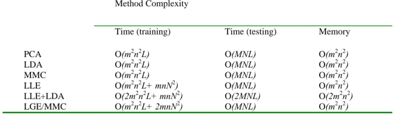
In Table 1, we compare the computational and the memory space complexities of the six methods. Here m and n is the number of the rows and the columns of the image matrix. L, M and N are the number of the projection vectors, the testing and the training samples, respectively.

Table 1: The computational and the memory space complexities of the six methods. Method Complexity

Time (training) Time (testing) Memory

PCA O(m2n2L) O(MNL) O(m2n2) LDA O(m2n2L) O(MNL) O(m2n2) MMC O(m2n2L) O(MNL) O(m2n2) LLE O(m2n2L+ mnN2) O(MNL) O(m2n2)

LLE+LDA O(2m2n2L+ mnN2) O(2MNL) O(2m2n2)

LGE/MMC O(m2n2L+ 2mnN2) O(MNL) O(m2n2)

In Table 1, for the PCA, LDA and MMC, since we need to perform O(MN) tests when using the nearest neighbour rule for classification and for each test it has the time complexity of O(L), the testing time is O(MNL). The memory cost is determined by the size of the matrices of the associated eigen equations, which is O(m2n2). The training time complexity depends on both the size of the matrices in the eigen equations and the number of the projection vectors that are required to be computed, which is O(m2n2L). For the LLE method, an extra time cost to construct the similarity matrix, i.e., O(mnN2), will be taken into account. So, LLE+LDA has the time complexity of O(2m2n2L+ mnN2), the testing time is O(2MNL) and Memory is O(2m2n2). The proposed method LGE/MMC has the time complexity of O(m2n2L+ 2mnN2), the testing time is O(MNL) and Memory is O(m2n2). So the proposed method is much than other methods in testing time.

6

Experiments and results

To evaluate the proposed LGE/MMC algorithm, we systematically compare it with the PCA [1], LDA [2], LLE [8-9], MMC [33] and LLE+LDA [23-24] algorithm in three face databases: ORL, YALE and AR. When the projection matrix was computed from the training part, all the images including the training part and the test part were projected to feature space. Euclidean distance and nearest neighborhood classifier are used in all the experiments. The experiments were carried out on the same PC (CPU: P4 2.8 GHz, RAM: 1024 MB).

6.1

Database

tolerance for some tilting and rotation of the face of up to 20 degrees. Moreover, there is also some variation in this scale of up to about 10 percent. All images normalized to a resolution of 56×46. We test the recognition performances of the six methods: PCA, LDA, LLE, MMC, LLE+LDA and LGE/MMC. In the experiments,

l

images (

l

varies from 2 to 6) are randomly selected from the image gallery of each individual to form the training sample set. The remaining

10



l

images are used for testing. For each

l

, we independently run 50 times. In the PCA phase of LDA, LLE, MMC, LLE+LDA and LGE/MMC, we keep 95 percent image energy.

The YALE face database [35] contains 165 gray scale images of 15 individuals, each individual has 11 images. The images demonstrate variations in lighting condition, facial expression (normal, happy, sad, sleepy, surprised, and wink). In this experiment, each image in Yale database was manually cropped and resized to 50×40. In the PCA phase of LDA, LLE, MMC, LLE+LDA and LGE/MMC, we keep 95 percent image energy. In the experiments,

l

images (

l

varies from 2 to 6) are randomly selected from the image gallery of each individual to form the training sample set. The remaining

11



l

images are used for testing. For each

l

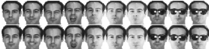
, we independently run 50 times.

The AR face database [36] contains over 4,000 color face images of 126 people (70 men and 56 women), including frontal views of faces with different facial expressions, lighting conditions, and occlusions. The pictures of 120 individuals (65 men and 55 women) were taken in two sessions (separated by two weeks) and each section contains 13 colour images. The face portion of each image is manually cropped and then normalized to 50×40 pixels. These images vary as follows: 1. neutral expression 2. smiling 3. angry 4. screaming 5. left light on 6. right light on 7. all sides light on 8. wearing sum glasses 9. wearing sun blasses and left light on 10. wearing sun blasses and right light on. In this experiment,

l

images (

l

varies from 2 to 6) are randomly selected from the image gallery of each individual to form the training sample set. The remaining

20



l

images are used for testing. For each

l

, we independently run 10 times. In the PCA phase of LDA, LLE, MMC, LLE+LDA and LGE/MMC, the number of principle components is set as 150. The dimension steps are set to be 5 in final low-dimensional subspaces obtained by the seven methods.

Fig.1, Fig.2 and Fig.3 show the sample images from the three databases.

Fig.1 Images of one person on the ORL database

Figure 2: Images of one person on the YALE database.

Figure 3: Images of one subject of the AR database. The first line and the second line images were taken in different time (separated by two weeks).

6.2

Experimental results and analysis

Except PCA and LDA, the local methods involved in the experiments are manifold learning based approaches, where

K

_c and

K

_p nearest neighbourhood search are contained. Thus how to select

K

_c and

K

_p are an important problem in feature extraction. If the value of

c

K

and

K

_pare too small, it is very difficult to preserve the topologic structure in low-dimensional space. On the contrary, if the value of

K

_cand

K

_pare too big, it is very difficult to depict the assumption of local linearity in high dimensional space. So it will affect the dimensionality manifold reduction result by the value of

K

_cand

K

_p. In the first experiment, we investigate the performance of the LGE/MMC algorithm over the reduced dimensions versus the corresponding varied the value of

K

_cand

K

_p. To find how

K

_cand

K

_paffect the recognition performance, we change

k

_c

 

l

1

and

p

K

are from 1 to 20 with step 1. Fig.4 displays the

average recognition rates with varied the value of

K

_pby carrying out LGE/MMC when only two images per class were randomly selected for training on the YALE face databases. LGE/MMC obtains the best average recognition rate is 94.79% when

K

_p=4. This indicates that the locality and the globality are with the same importance. In the next experiment, the value of adjustable parameter

K

_pis taken to be 4.

p

K

when only two images per class were randomly selected for training on the YALE face databases.

In the second experiment, we also test the impact of



on the performance when only two images per class were randomly selected for training on the YALE face database, which can be found in Fig. 5. We varied



from 1 to 100 with step 1. Fig. 5 displays the maximal average recognition rates with varied parameter



by carrying out LGE/MMC. From Fig. 5, it can be found that the effectiveness of the LGE/MMC algorithm is sensitive to the value of the parameter



. LGE/MMC obtains the best average recognition rate is 94.79% when



=6. This indicates that the locality and the globality are with the same importance. In the next experiment, the value of adjustable parameter



is taken to be 6.

In the third experiment, we randomly select

l

images (

l

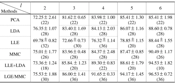
varies from 2 to 6) of each individual for training, and the remaining ones are used for testing. We compare the performances of different algorithms. The average recognition rates obtained by different algorithms as well as the corresponding dimensionality of reduced subspace (the numbers in parentheses) on the ORL, YALE and AR face databases are given in the Table 2, Table 3 and Table 4, respectively. Fig.6. is the average recognition rates (%) of LGE/MMC versus the corresponding varied dimensions when only six images per class were randomly selected for training on the ORL, YALE and AR face databases. We change the number of eigenvectors from 2 to 50 with step 2 on the ORL, YALE face databases and the number of eigenvectors from 5 to 150 with step 5 on the AR face database, respectively.

Table 2: The average recognition accuracy(%)of different algorithms on the ORL face database and the corresponding standard deviations and dimensions.

l

Methods 2 3 4 5 6

PCA 72.25



2.61

(22)

81.62



0.65 (22)

83.98



1.00 (22)

85.41



1.30 (22)

85.41



1.98 (22)

LDA 76.35



1.07

(28)

83.40



1.69 (28)

84.13



2.03 (28)

86.07



1.16 (28)

88.60



0.78 (28)

LLE 69.78



0.82

(32)

72.66



0.73 (30)

76.32



1.14 (36)

78.85



1.15 (20)

88.44



1.55 (28)

MMC 75.01



1.77

(26)

83.96



0.48 (28)

84.37



2.48 (28)

87.47



0.85 (28)

90.49



1.17 (26)

LLE+LDA 73.36



1.24

(18)

85.84.



1.23 (20)

89.30



0.83 (22)

88.61



1.79 (20)

94.53



1.82 (10)

LGE/MMC 75.53



1.88

(30)

86.00



1.41 (36)

91.65



0.33 (36)

94.17



1.45 (36)

96.53



0.72 (36)

Table 3: The average recognition accuracy(%) of different algorithms on the YALE face database and the corresponding standard deviations and dimensions.

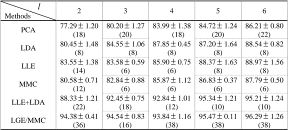
Table 4: The average recognition accuracy(%) of different algorithms on the AR face database and the corresponding standard deviations and dimensions.

l

Methods 2 3 4 5 6

PCA 66.68



1.11

(85)

70.21



1.62 (85)

77.60



1.27 (85)

79.03



0.81 (80)

81.54



1.04 (85)

LDA 71.50



0.71

(70)

75.58



0.76 (70)

82.53



0.81 (70)

87.12



0.33 (70)

87.58



0.75 (70)

LLE 70.40



0.89

(85)

74.31



1.16 (75)

83.35



1.49 (70)

84.78



0.76 (80)

86.98



0.40 (85)

MMC 69.39



1.15

(80)

75.71



0.59 (80)

82.98



0.62 (85)

85.27



0.94 (80)

87.86



0.82 (80)

LLE+LDA 69.38



1.20

(90)

79.23



0.89 (80)

88.17



1.36 (80)

89.09



1.49 (85)

92.420



1.08 (80)

LGE/MMC 71.99



0.99

(75)

81.00



0.78 (50)

90.46



0.89 (85)

91.39



0.91 (45)

95.60



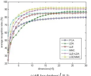
0.80 (50)

(a)ORL face database(

l



4 ) (b) Yale face database(

l



6)

l

Methods 2 3 4 5 6

PCA 77.29



1.20

(18)

80.20



1.27 (20)

83.99



1.38 (18)

84.72



1.24 (20)

86.21



0.80 (22)

LDA 80.45



1.48

(8)

84.55



1.06 (8)

87.85



0.45 (8)

87.20



1.64 (8)

88.54



0.82 (8)

LLE 83.55



1.38

(14)

83.58



0.59 (6)

85.90



0.75 (6)

88.37



1.63 (8)

88.97



1.56 (8)

MMC 80.58



0.71

(12)

82.84



0.88 (6)

85.87



1.12 (6)

86.83



0.37 (6)

87.79



0.50 (6)

LLE+LDA 88.33



1.21

(22)

92.45



0.75 (18)

92.84



1.01 (12)

95.34



1.21 (10)

95.21



1.24 (10)

LGE/MMC 94.38



0.41

(36)

94.54



0.83 (16)

93.84



1.16 (38)

95.47



0.11 (38)

(c)AR face database(

l



5)

Figure 6: The average recognition rates (%) of LGE/MMC versus the corresponding varied dimensions on the ORL, YALE and AR face databases.

The above experiments showed that the maximal average recognition rates of all methods increases with the increase in training sample size in Table 2, Table 3 and Table 4 respectively. The proposed LGE/MMC algorithm consistently outperforms better than other methods in all experiments in three face databases. From Fig.6 we can find that with the increase number of eigenvectors on three face databases, the average recognition rates also improved.

7

Conclusions

In pattern recognition, feature extraction techniques are widely employed to reduce the dimensionality of data and enhance the discriminatory information. In this paper, we proposed a new method for feature extraction and recognition, namely local graph embedding method based on maximum margin criterion (LGE/MMC) for dimensional reduction. The results of face recognition experiments on ORL, YALE and AR face databases demonstrate the effectivity of the proposed method. In the future, we will make more tests on other types of data and decide the optimal parameter



,

K

_c and

K

_p. For future work, we will extend LGE/MMC to supervised and semi-supervised cases.

Acknowledgements

This work is partially supported by the National Science Foundation of China under grant no. 60632050, 90820306, 60873151, 60973098, 61162002, 61005008, 61005005, 60963002, the National Science Foundation of Jiangxi Provincial under grant no. 20114BAB201034, China's Aviation Science no. 20115556007 and Youth Foundation of Jiangxi Provincial Department of Education no. GJJ12459.

References

[1] M. Turk, A.P. Pentland (1991) Face recognition using eigenfaces. In: Proceedings of IEEE

Computer Society Conference on Computer Vision and Pattern Recognition, Maui, Hawaii, June 1991, pp. 586–591

[2] P.N. Belhumeur, J.P. Hespanha, D.J. Kriengman (1997) Eigenfaces vs. Fisherfaces: recognition using class specific linear projection. IEEE Trans. Pattern Anal. Mach. Intelligence 19(7): 711–720 [3] M. Kirby, L. Sirovich (1990) Application of the KL

procedure for the characterization of human faces. IEEE Transactions on Pattern Analysis and Machine Intelligence 12(1): 103–108

[4] [4] J.M. Lee (1997) Riemannian Manifolds: An Introduction to Curvature. Springer, Berlin

[5] B. Scholkopf, A. Smola, K.R. Muller (1998) Nonlinear component analysis as a kernel eigenvalue problem. Neural Comput 10 (5): 1299– 1319

[6] S. Mika, G. Ratsch, J. Weston, B. Scholkopf, A.

Smola, K.-R. Muller (2003) Constructing

descriptive and discriminative nonlinear features: Rayleigh coefficients in kernel feature spaces. IEEE Trans. Pattern Anal. Mach. Intell. 25(5): 623–628. [7] J.B. Tenenbaum, V. de Silva, J.C. (2000) Langford

A global geometric framework for nonlinear dimensionality reduction. Science 290(5500): 2319–2323.

[8] S.T. Roweis, L.K. Saul (2000) Nonlinear dimensionality reduction by locally linear embedding. Science 290(5500): 2323–2326.

[9] L.K. Saul, S.T. Roweis (2003) Think globally, fit locally: unsupervised learning of low dimensional manifolds. J. Mach. Learn. Res 4: 119–155.

[10] M. Belkin and P. Niyogi, T. G. Dietterich, S. Becker, and Z. Ghahramani (2000) Laplacian eigenmaps and spectral techniques for embedding and clustering. Advances in Neural Information Processing Systems 14: 873-878

[11] M. Belkin, P. Niyogi (2003) Laplacian eigenmaps

for dimensionality reduction and data

representation. Neural Comput 15(6): 1373–1396. [12] Z. Zhang, H. Zha (2004) Principal manifolds and

nonlinear dimensionality reduction via tangent space alignment. SIAM Journal of Scientific Computing 26(1): 313–338

[13] X. He and P. Niyogi (2003) Locality Preserving Projections. In: Proceedings of the 17th Annual Conference on Neural Information Processing

Systems, Vancouver and Whistler, Canada,

December 2003, pp. 153-160

[14] X. He, S. Yan, Y. Hu, P. Niyogi, and H.-J. Zhang (2005) Face Recognition Using Laplacianfaces. IEEE Trans. Pattern Analysis and Machine Intelligence 27(3): 328-340

[15] H. Hu (2008) Orthogonal neighborhood preserving discriminant analysis for face recognition. Pattern Recognition 41: 2045–2054.

[16] W. Yu, X. Teng, C. Liu (2006) Face recognition using discriminant locality preserving projections. Image Vision Computing 24: 239–248

projections for face recognition. Neurocomputing 71: 3644–3649

[18] G. F. Lu, Z. Lin, Z. Jin (2010) Face recognition using discriminant locality preserving projections based on maximum margin criterion. Pattern Recognition 43: 3572-2579

[19] D. de Ridder, R.P.W. Duin, Locally linear embedding for classification, Technical Report PH-2002-01, Pattern Recognition Group, Department of Imaging Science and Technology, Delft University of Technology, Delft, The Netherlands, 2002. [20] D. de Ridder, O. Kouropteva, O. Okun, M.

Pietik¨ainen, R.P.W. Duin, Supervised locally linear embedding, artificial neural networks and neural information processing, in: ICANN/ICONIP 2003 Proceedings, Lecture Notes in Computer Science, vol. 2714, Springer, Berlin, 2003, pp. 333–341. [21] X. Bai, B. Yin, Q. Shi, Y. Sun, Face recognition

based on supervised locally linear embedding method, J. Inf. Comput. Sci. (4) (2005) 641–646. [22] O. Kouropteva, O. Okun, M. Pietikainen,

Supervised locally linear embedding algorithm for pattern recognition, IbPRIA 2003, Lecture Notes in Computer Science, vol. 2652, Springer, Berlin, 2003, pp. 386–394.

[23] J. Zhang, H. Shen, Z.-H. Zhou, Unified Locally Linear Embedding and Linear Discriminant Analysis Algorithm for Face Recognition, Lecture Notes in Computer Science, Springer, Berlin, 2004. [24] J. Zhang, H. Shen, Z.-H. Zhou, Ensemble-based

discriminant manifold learning for face recognition, ICNC 2006, Part I, Lecture Notes in Computer Science, vol. 4221, Springer, Berlin, 2006, pp. 29– 38.

[25] X.F. He, D. Cai, S.C. Yan, H.J. Zhang (2005)

Neighborhood preserving embedding. In:

Proceedings of IEEE International Conference on Computer Vision (ICCV), Beijing, china, October 2005, pp. 1208–1213.

[26] X.H. Zeng, S.W. Luo (2007) A supervised subspace learning algorithm: supervised neighborhood preserving embedding. In: Proceedings of 3rd

International Conference on Adwanced Data Mining and Applications, Harbin, China, August 2007, pp 81-88

[27] Y. Wang, Y. Wu (2010) Complete neighborhood preserving embedding for face recognition. Pattern Recognition 43:1008-1015

[28] C. Hwann-Tzong, C. Huang-Wei, L. Tyng-Luh, Local discriminant embedding and its variants, in: Proceedings of the 2005 IEEE Computer Society Conference on Computer Vision and Pattern

Recognition (CVPR'05) - Volume 2 (IEEE

Computer Society, 2005).

[29] S.C. Yan, D. Xu, B.Y. Zhang, H.J. Zhang, Q. Yang, S. Lin, Graph embedding and extensions: A general framework for dimensionality reduction, IEEE Trans. Pattern Anal. Mach. Intell. 29 (2007) 40-51. [30] P.Y. Han, A.T.B. Jin, F.S. Abas, Neighbourhood

preserving discriminant embedding in face

recognition, J. Vis. Commun. Image Represent. 20 (2009) 532-542.

[31] M.A. Turk, A.P. Pentland, Face recognition using eigenfaces, IEEE Computer Society Conference on

Computer Vision and Pattern Recognition

(91CH2983-5), (1991).

[32] S. Yan, D. Xu, B. Zhang, and H.-J. Zhang, Graph

Embedding: A General Framework for

Dimensionality Reduction, IEEE Computer Society Conference on Computer Vision and Pattern Recognition(CVPR’05), vol. 2, pp. 830-837, 2005, San Diego.

[33] H. Li, T. Jiang, K. Zhang, Efficient and robust feature extraction by maximum margin criterion, IEEE Transactions on Neural Networks 17 (1) (2006) 1157–1165.

[34] AT&T Laboratories Cambridge, The ORL database

of faces, _http://www.uk.research.att.com/

facedatabase. Html.

[35] Yale database, 1997. Available from:

<http://cvc.yale.edu/projects/yalefaces/yalefaces.ht ml>.