Two-phase Simulation of Well Control Methods for Gas Kicks in Case of Water and Oil-based Muds

(1)

http://jpst.ripi.ir Journal of Petroleum Science and Technology 2018, 8(4), 34-48

ABSTRACT

Kick occurrence is a possible event during a drilling process. It is required to be handled immediately using a well control method to avoid blowout, financial losses and damages to the drilling crew. Several methods including driller, wait and weight, and concurrent are applicable in the drilling industry to control a well during a kick incident. In this study, typical well control methods were simulated for both cases of water and oil-based muds, and essential parameters such as the required time were calculated. Additionally, for each well control approach, a mathematical algorithm was proposed to simulate the process. In case of oil-based mud, the flash calculation was utilized in each depth and time by considering the effect of kick fluid dissolution in drilling mud to improve the accuracy of control parameters. Based on the results, when oil-based mud is used for drilling, extra time is required to control the well due to kick fluid dissolution in the mud and extensive changes in the mud density. In order to improve the accuracy of the calculations, critical parameters including temperature changes in the well column, dynamic drilling hydraulics, and pressure drop were considered during a well control process. In addition, the simulation of the concurrent method is one of the study innovations because of mud density alternations especially when the mud becomes heavier by a non-linear or complicated mathematical function during the process.

Keywords: Well control, Two-Phase, Simulation, Water and Oil Based Muds. Yaser Jahanpeyma and Saeid Jamshidi*

Chemical and Petroleum Engineering Department, Sharif University of Technology, Tehran, Iran

Two-phase Simulation of Well Control Methods for Gas Kicks in Case

of Water and Oil-based Muds

*Corresponding author Saeid Jamshidi

Email: [email protected] Tel: +98 21 6616 6412 Fax: +98 21 6616 6412

Article history

Received: August 09, 2017

Received in revised form: December 26, 2017 Accepted: January 22, 2018

Available online: December 01, 2018 DOI: 10.22078/jpst.2018.2834.1471

INTRODUCTION

Kick is a prevalent problem during a large number of drilling operations in which the formation fluid enters the wellbore as a result of higher pressure of formation relative to hydrostatic pressure. Gas type kicks are more commonplace than liquid types. In order to specify kick type, kick fluid density should be estimated using drilling parameters such as Shut-in Drill Pipe Pressure (SIDPP), Shut-in Casing Pressure (SICP) and depth. Due to the fact that gas

kicks have more complicated behavior than the liquids, and are more challenging to be controlled, usually, a gas type is assumed for kick fluid in a well control simulation.

(2)

In all the mentioned methods, bottom-hole pressure should remain constant during the operation by means of alternating pump speed and choke opening and closing. Furthermore, it is possible for the crew to close the choke, and survey the well conditions in any step of the operation. The final pressure should remain constant when the new mud reaches to the drill bit at the bottom-hole. Choe [1] analyzed well control process applying mass and momentum balance and auxiliary equations for liquid and gas phases in order to calculate density and gas speed values in any region of the well. The analysis contained only water-based mud condition based on the assumption of non-solubility of kick fluid in the drilling mud. He analyzed kick occurrence condition in the Gulf of Mexico.

Avelar et al [2] simulated well control process for newly discovered fields in Brazil. They simulated the process for gas kick type and water-based mud using mass and momentum balance and auxiliary equations. Omosebi et al. [3] analytically predicted annulus pressure during a kick occurrence. They used flash calculations for oil-based muds and assumed that the kick fluid may move as a slug or may be mixed with the drilling fluid. However, they did not consider the effects of gas dissolution in the mud. Marbun and Shidiq [4] calculated annulus and casing shoe pressure during a well control process. They supposed that the gas expands when rising from bottom-hole to the surface with the assumption of non-solubility of gas in the kick fluid. An et al. [5] simulated kick behavior in high-pressure high-temperature conditions in offshore wells filled with oil-based muds. They realistically modeled wellbore pressure profile and kick behavior using their proposed method. Results showed that mud density decreases as well depth increases due

to the fact that the temperature effect is more dominant relative to the pressure.

An advanced simulator for predicting standpipe and choking pressure in deep water horizontal well killing based on dynamic bottom-hole pressure was developed by Feng et al [6]. The simulator is able to simulate driller’s method considering circulation temperature, gas expansion and choke line friction losses. A gas kick incident was simulated by Sun et al, and a well killing was conducted a dynamic hydraulic simulator using transient multiphase flow model for a high-pressure high-temperature well in western China by Sun et al [7]. The simulation revealed underlying physics and causes of several intriguing phenomena and calculated an appropriate pump rate in order to kill the well successfully.

(3)

Journal of Petroleum Science and Technology 2018, 8(4), 34-48 http://jpst.ripi.ir

EXPERIMENTAL PROCEDURES

Materials and Methods

Operational approach of the three well control methods contains running new mud (which is heavier than the initial one) into the well. In driller’s method, the prepared mud is pumped into the well after running out the initial (two circulations). In the wait & weight method, the new mud is pumped into the well simultaneously as the initial mud is running out (one circulation). In the concurrent method, the mud weight is increased stepwise in contrast to other methods; the heavier mud is pumped into the well at each step of mud preparation until reaching to the surface [12-14].

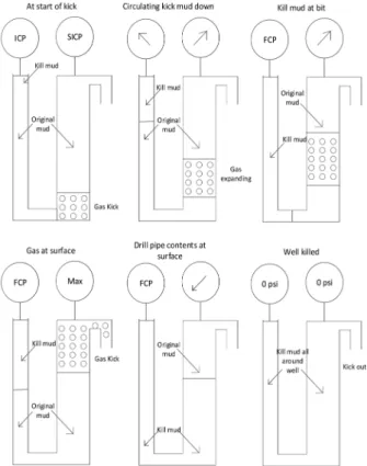
The Driller’s Method

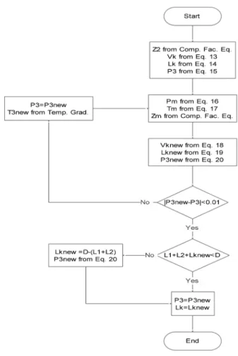
Driller’s method, whose procedure has been represented in Figure 1, is a practical well control approach in the drilling industry because of uncomplicated operation [12].

Figure 1: Driller’s method procedure.

The Wait & Weight Method

In this method, the heavier mud preparation is started immediately after the kick occurrence and then pumped into the well. The initial mud is withdrawn from the mud circulation system and simultaneously is substituted by a heavier mud until reaching to the surface [12]. Figure 2 illustrates the stepwise procedure of wait & weight method.

Figure 2: Wait & weight method procedure.

(4)

The Concurrent Method

This method is utilized whenever strong kicks or mud loss take place in the well, in which pump speed should remain at the minimum rate, and mud density is gradually increased.

The major advantage of the concurrent method is that casing pressure is lower compared to the other two methods due to fewer damages to the equipment arising from incremental mud weight increasing. However, the method is more complicated than the others and requires further facilities on the rig.

The procedure of concurrent methods includes: 1- After closing the well and data recording, required parameters such as ICP, FCP are calculated.

2- The pump is turned on and brought up to kill rate speed while casing pressure is held constant. When the pump reaches the kill rate, drill pipe pressure is adjusted to the calculated value. Circulation should be started as soon as ICP is determined.

3- Mud pit crew should increase mud weight during circulation. Whenever mud weight increases to a value at the bottom of the chart, choke operator adjusts circulating pressure to the drill pipe pressure. 4- Circulating is continued until kill weight mud comes back to the surface. [12].

Well Control Simulation for

Water-Based Muds

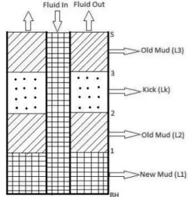
In this study, kick fluid and water-based mud are not supposed to mix or dissolve in each other. Hence, drill string fluid column consists of two layers including old and new mud. Annulus fluid column is composed of four layers: (from bottom to top) new mud, old mud, kick fluid and old mud, schematically displayed in Figure 3. Due to fluid displacement in the well column, the height and

boundaries of the layers are changing during the process [15-16].

Figure 3: Fluid layers in the well during the well control process.

Equations 1-33 were utilized in order to calculate well control parameters to be used in the flowchart of each method (Figure 4 to Figure 9). The definitions of the parameters are available in the nomenclature section.

Firstly, the basic parameters specially required time of each method is calculated. The required time for passing through the string and annulus are respectively calculated by Equations 1 and 2, and their summation in Equation 3.

s s

V t

SCR

= (1)

a a

V t

SCR

=

(2)

3 0 a

t =t +t (3)

In Equations 4, 5 and 6, the elapsed time of each well control method has been calculated using Equations 1, 2 and 3.

3

driller a

t = +t t (4)

& 3

wait weight w

(5)

Journal of Petroleum Science and Technology 2018, 8(4), 34-48 http://jpst.ripi.ir min 3

concurrent

t =t +t (6) The lengths of some sections of Figure 3, which separate different parts of the well versus fluid type, are calculated by Equations 7, 8 and 9.

( _a)

n

s

SCR t t CF L

A

−

= ₍₇₎

2

a

SCR t CF L

A

× ×

= (8)

1

( ( a) )

a

s

SCR t t V L

A

CF

− −

= (9)

Pressure values at critical points especially boundaries of fluid layers and surface are calculated using Equations 10, 11 and 12.

0.052 0.052

ss BH o n s b

P P= − ×MW L× − ×KMW L× + ∆ + ∆ −P P SCP

(10)

1 BH 0.052 1

P P= − ×KMW L× ₍₁₁₎

2 1 0.052 2

P =P − ×MW L× (12) Kick fluid properties such as volume, length and top pressure are calculated using trial and error procedures based on the Equations 13 to 20 due to the variable volume of gaseous kick fluid and its expansion when rising toward the surface. Afterward, the constant surface pressure could be calculated by Equation 21. The procedure flowchart has been illustrated in Figures 8 and 9.

2

BH kBH

k

BH

P z V V

P z

= (13)

k k a V CF L A

= ₍₁₄₎

3 2

2 2

( )

1544 k ML

P P EXP

z T

−

= (15)

2 3

2

m P P

P = + (16)

2 3

2

m T T

T = + (17)

BH m kBH

knew

m BH

P z V V

P z

= (18)

knew knew a V CF L A

= ₍₁₉₎

3new 2 . (₁₅₄₄ knew )

m m

ML

P P EXP

z T

−

= ₍₂₀₎

3 0.052 3

s

P =P − ×MW L× (21)

1 2

( _k)

KTP D L L L= − + + (22)

In the wait and weight method, gas rising velocity during the waiting period of the procedure is calculated using Equation 24. Other formulations in Equations 23 to 28 can be utilized in order to calculate the lengths of fluid sections in Figure 3.

( w)

n

s

SCR t t CF L

A

−

= ₍₂₃₎

0.101 L G

gr t

L

V gr ρ ρ

ρ

−

= (24)

2 gr

L V t= (25)

2 ( w) gr w a

SCR t t CF L

A V t

−

= + (26)

1

( ( w) )

a s

SCR t t V

L

A

CF

− −

= (27)

2 s gr w a

V CF L

A V t

= + ₍₂₈₎

Equations 29 to 33 are used to calculate the lengths of sections in Figure 3 for the concurrent method. The expression g(t) in Equation 29 represents the mathematical function of mud weight changes and its average value. The pressure parameter in the boundaries and kick fluid behavior are the same as the driller and wait & weight methods.

( ) ( , ) f i t t i f f i

g t dt f t t

t t = −

∫

(29) n s SCR t CF L

A

× ×

= ₍₃₀₎

2

a

SCR t CF L

A × ×

(6)

1

( )

a s

SCR t t CF L

A −

= ₍₃₂₎

2 a s

V CF L

A

= ₍₃₃₎

Figures 4, 5 and 6 exhibit the procedure of principal flowcharts of the three methods by which required parameters could be computed at any desired time during well control process. In order to complete the simulation, calculations should be performed at different time intervals from zero to maximum elapsed time of the process. For instance, the required time for driller’s method was calculated 226.63 minutes in this study. The interval (0-226.63) could be divided by 100 time steps, in addition, at any of them, these calculations could be performed to compute major parameters including annular surface pressure, casing shoe pressure, etc.

The procedures of several critical parameters such as casing shoe pressure, kick top depth, kick region length, surface pressure, etc. are the same for the three methods of well control which are stated in Figure 7 along with the general section of the methods.

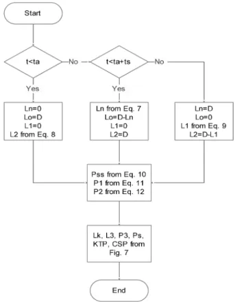
Based on the computational procedure of driller’s method in Figure 4, there are three time intervals whose formulations are different from each other. -t<t_a: the period before bottom-hole fluid reaches to the surface

-t<t_a+t_s: the period before heavier mud reaches to the end of the string

-else (other times): the period that heavier mud moving from string bottom to the surface through the annulus

For each of the time intervals, the lengths of the fluid sections and their pressure in boundaries and internal sections have been calculated.

Figure 4: the Computational procedure of driller’s

method.

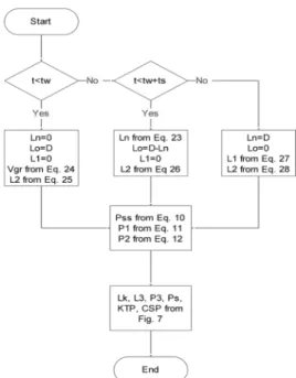
Similar to the driller’s method, a computational procedure has been proposed for the wait & weight method in Figure 5. There are three time intervals for simulation based on the mechanism of the method:

-t<t_w: the period that the crew are preparing the new mud

-t<t_w+t_s: the period in which new mud is prepared and is pumped to the string, although has not reached to the bottom

-else (other times): the period in which new mud entering the annulus, before reaching to the surface.

(7)

Figure 5: The Computational procedure of wait & weight

method.

A computational procedure has been proposed for the concurrent method in Figure 6 based on which three time intervals exist:

-t<t₀: the period before mud weight reaches to the final weight from the initial weight.

-t<t₃: the period before the complete exit of old mud (which is under kick fluid)

-else (other times): before the final mud completely entering the annulus

The procedure of calculating the major parameters such as kick fluid properties and pressure at critical points of the well, especially boundary of fluid layers is the same in all the three well control methods. Figure 7 illustrates the general section in which different procedures and equations have been proposed for both water and oil-based muds because kick region properties such as length, volume and pressure are different depending on the mud type.

Figure 6: the Computational procedure of the concurrent

method.

Figure 7: Computational procedure for the general part of the three methods.

(8)

Figure 8: the Computational procedure of kick fluid region for water-based muds.

Oil-based muds consist of diesel as a continuous phase and water as a discontinuous phase. A chemical emulsifier is added to the mixture in order to prevent water droplets from joining and sticking together [9]. Diesel density at 60 F is 820-860 kg/m3_{, and it approximately contains hydrocarbons}

in the range of C₁₀ to C₁₅ [17].

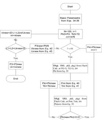
Figure 9 illustrates well control stages for oil-based muds. Due to the fact that kick fluid mostly contains hydrocarbon gas (methane) and oil-based muds contain hydrocarbon fluids, it could be supposed that the entered gas is soluble in the drilling fluid [18]. Therefore, there is a new kick fluid combination whose composition is lighter than the original diesel and is moving toward the surface.

Thus, it may be converted into two phases during the process, and so, flash calculations are required for computing its properties. PR78 was utilized as the equation of state, and Simultaneous Solution Method (one of the flash calculation methods) for two-phase analysis [19-21]. Also, the mud includes diesel and solid particles which are calculated by Equations 34 to 36 have been considered in the calculations.

Based on the procedure details in Figure 9, the kick fluid is discretized to 100 equal sections. Gas and liquid volumes and hydrostatic pressure of each section are calculated using a try and error procedure combined with flash calculation.

w w l

V =x V ₍₃₄₎

d d l

V =x V (35)

s s l

V =x V (36)

The new molar amounts of each component and their fractions in the new kick fluid are calculated using Equations 37 and 38.

20

1 14

t c ci

i

n n n =

= +

∑

₍₃₇₎

( 1, 14 20)

i i

t

z n i

n = −

= (38)

Pressure, volume and length of kick fluid in case of oil-based muds are calculated using Equations 39 to 43.

( 1) ( )

ki k i kgi kgi kli kli

c a

gCF

P P V V

g A ρ ρ

−

= − − ₍₃₉₎

( 1)

2

k i ki

mi

P P

P ₌ − + ₍₄₀₎

( 1)

2

k i ki

mi

T T

T ₌ − + ₍₄₁₎

1 1

N N

k kgi kli w s

i i

V V V V V

= =

=

∑

+

∑

+ + ₍₄₂₎

k k

a

V CF L

A

(9)

Figure 9: The Computational procedure of kick fluid region for oil-based mud.

RESULTS AND DISCUSSIONS

In this section, the well control process has been simulated for water and oil-based muds. Tables 1 and 2 contain the input data used in the simulation.

Table 1: Input data for water-based mud. Input parameter (unit) Value

Depth (ft) 10000

Mud Weight (ppg) 9.6 Casing Shoe Depth (ft) 3500 Shut In Drill Pipe Pressure (psig) 720 Shut In Casing Pressure (psig) 520 Input Kick Volume (bbl) 20

Table 2: Input data for oil-based mud. Input parameter (unit) Value

Depth (ft) 5000

Mud Weight (ppg) 7.2 Casing Shoe Depth (ft) 3500 Shut In Drill Pipe Pressure (psig) 250 Shut-In Casing Pressure (psig) 150 Input Kick Volume (bbl) 20

Simulation Results for Water-Based Muds

According to Table 3, the required time for controlling the well by the concurrent method is shorter than wait & weight, and wait & weight’s method time is shorter than the driller’s method time. Therefore, the concurrent method is more economical relative to the other methods for controlling the well.

Table 3: Input data for oil-based mud.

Well Control Method Time (min)

Driller 226.63

Wait & weight 159.26

Concurrent 140.88

In Figure 10, annular surface pressure versus time has been displayed for the three methods. In drillers’ method, due to the expansion of rising gas in well column, the pressure increases until the kick fluid reaches the surface. During gradual gas withdrawal, the annular pressure is reducing until the gas exit completely from the well, and after that, the new mud is entering into the well. The pressure remains constant during new mud entrance to the annulus, and after which, the pressure is reducing until the annulus eventually occupied by the new mud.

Time (min)

Annular surf

ace pr

essur

e (p

si)

Figure 10: Annular pressure vs. time for water-based

(10)

In wait & weight method, the pressure increases during the waiting period as a consequence of gas rising in the well column especially due to extensive expansion near the surface. When heavy mud enters the annular space, the pressure starts to reduce. During gradual gas withdrawal, the pressure is quickly decreasing until complete replacement of heavy mud.

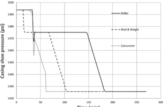
The procedure of concurrent method is similar to the wait & weight except that due to the gradual change of mud weight, the trend of the graph is not linear in some areas. Figure 11 shows casing shoe pressure versus time for the three methods. As long as the gas is moving upward and expanding, the casing shoe pressure is decreasing. When kick fluid passes through the casing shoe, the pressure is decreasing. Until the new mud enters the annulus, the casing shoe pressure remains constant in driller’s method and decreases in the others because of new mud weight effects. The casing shoe pressure, which is a critical parameter during the drilling process, remains constant at the end of the process and complete substitution of the new mud.

Time (min)

Casing shoe pr

essur

e (p

si)

Figure 11: Casing shoe pressure vs. time for water-based muds.

Figure 12 illustrates surface drill pipe pressure versus time for driller’s and wait & weight methods in which the pressure remains constant until the arrival of new mud. In this stage, firstly the pressure

Time (min)

Su

rf

ace pi

pe pr

essur

e (

psi

)

Figure 12: Surface drill pipe pressure vs. time for water-based muds.

The three methods do not have considerable differences in the period of kick fluid arriving at the surface based on Figure 13 in which kick top depth has been plotted versus time. After kick fluid reaching to the surface, the annulus pressure is reducing and consequently, well control process could be run with more safety and confidence. is reducing and after complete displacement, remains constant. In the concurrent method, since the new mud enters from the start of the process, the pressure is reducing. It should be noted that the immediate alternations of the chart slope are due to the arrival of new mud to the annulus.

Time (min)

Ki

k t

op dep

th (

ft)

Figure 13: Kick top depth vs. time for water-based

(11)

Simulation Results for Oil-Based Muds

The simulation results of oil-based muds have been presented in Table 4. The Table compares well control required times for the three methods. Similar to the water-based muds, the period of the concurrent method is shorter than wait & weight, and wait & weight than the drillers’. Therefore, the concurrent method is more economical relative to the other methods.

Table 4: Well control times for oil-based muds.

Well Control Method Time (min)

Driller 215.80

Wait & weight 192.31 Concurrent 169.34

Figure 14 illustrates annular surface pressure versus time for the three methods. In the driller’s method, the pressure remains constant whenever the kick fluid, composed of initial methane gas mixed with drilling fluid, contains only one phase. When the fluid contains two phases, the annular pressure is reducing until the kick fluid reaching to the surface. The pressure remains constant as long as new mud has not entered to the annulus. It should be noted that during gradual gas withdrawal of the well, the pressure starts to decrease to a final value of zero.

Time (min)

Annular surf

ace pr

essur

e (p

si)

Figure 14: Annular pressure vs. time for oil based muds.

Wait & weight method procedure is similar to drillers’ except no constant area in the graph due

Time (min)

Casing shoe pr

essur

e (p

si)

Figure 15: Casing shoe pressure vs. time for oil based

muds.

Figure 16 displays drill pipe pressure versus time whose general trend is similar to Figure 15. Two-phase fluid effect of annular fluid on drill pipe fluid is negligible, and consequently on the surface pipe pressure. to the new mud arrival. In the concurrent method, after the arrival of heavy mud into the annular space, the initial constant pressure is reducing. While the kick fluid contains two phases, the pressure decreases until kick fluid completely exit from the well. During the new mud entrance to the annulus, the pressure is decreasing to zeros. Figure 15 shows casing shoe pressure versus time for the three methods whose general trend is similar to Figure 14. The difference is in rapid changes in the graph when the kick fluid contains two phases.

Time (min)

Su

rf

ace pi

pe pr

essur

e (

psi

)

(12)

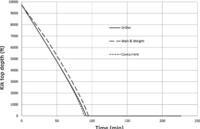
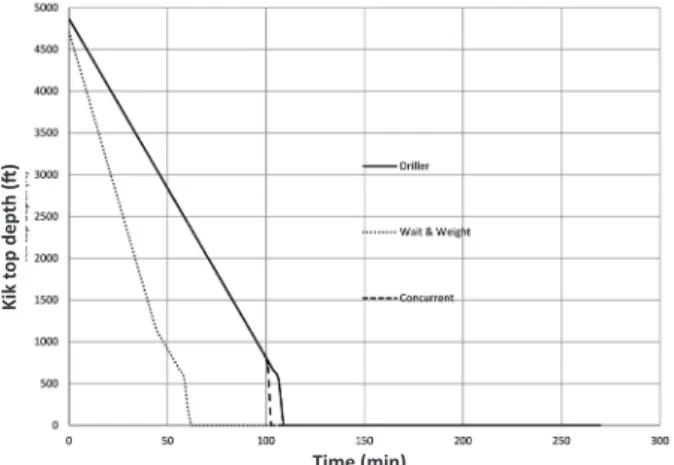
Figure 17 displays kick top depth versus time for oil based muds whose procedure for driller’s and concurrent methods are the same. However, the concurrent period for kick fluid reaching to the surface is shorter than the drillers’ due to single stages procedure. In wait & weight method, the kick fluid period for reaching to the surface is shorter than the others since during initial wait time when the well is shut in, the kick fluid is moving toward the surface. This difference is more obvious in oil-based muds since the wait time for preparing the oil-based muds are more considerable than the water-based muds.

Time (min)

Ki

k t

op dep

th (

ft)

Figure 17: Kick top depth vs. time for oil based muds.

RESULTS AND DISCUSSION

The major differences between the three methods are the approach of heavier mud substitution in the well and bringing out the kick fluid during which exerted pressure to the annulus at the well column is increasing. If the surface pressure could remain constant at a high value by BOP or other equipment, lower pressure will be exerted on the annulus and consequently, the risks and danger of operation will be decreased.

In the concurrent method, it is essential for the drilling crew to increase mud weight from initial to

the desired value at a short time, for example by an exponential function. However, this function is technically hard to be run because of equipment and technology limitations. This simulator is able to run the concurrent method using any desired function. It should be noted that the three methods have not considerable differences at the time of arriving the kick fluid to the surface.

It is important for a well control simulator to be run at a short time due to the fact that there is no time for the crew to wait for running the simulator in the actual condition. Maybe combining mass, momentum and energy balance equations could be another appropriate method to simulate the process. Nevertheless, needing extra running time is a disadvantage because of the finite difference or finite element method usage. In this study, simulation has been run at a shorter time relative to the others by flash calculation which is practical to be used in the actual conditions.

CONCLUSIONS

(13)

and the other equipment due to the fact that until complete kick fluid exit from the well, the casing shoe pressure has a large value, sometimes at a dangerous and destructive range.

In the case of oil-based muds, any changes in pressure and temperature have significant effects on the kick fluid behavior. Dissolution of kick fluid in drilling mud changes the mud density from bottom-hole to the surface, and consequently, more surface choke pressure will be required to maintain the bottom-hole pressure.

Another point about oil-based mud is that due to gas solubility in the kick fluid, the mud reaches later to the surface relative to water-based muds.

NOMENCLATURES

SIDPP: Shut in Drill Pipe Pressure, psi SICP: Shut in Casing Pressure, psi BOP: Blowout Preventer

ICP: Initial Circulation Pressure, psi FCP: Final Circulation Pressure, pi SCR: Slow Circulation Rate, bbl/min SCP: Slow Circulation Pressure, psi MW: Mud Weight, ppg

KMW: Kill Mud Weight, ppg KTD: Kick Top Depth, ft CSP: Casing Shoe Pressure, psi

CF: Conversion Factor (bbl to cubic ft), 5.615 L_n: Height of new mud in the drill string, ft L_o: Height of old mud in the drill string, ft

L₁: Height of new mud in the bottom of the annulus, ft

L₂: Height of old mud in annulus under the kick fluid, ft

L_k: Height of kick fluid in the annulus, ft

L₃: Height of new mud in the annulus above the kick fluid, ft

t_s: Required time for new mud to reach from the surface to bottom of the drill string, min

t_a: Required time for new mud to reach from bottom of the annulus to surface, min

t₁: Required time for old mud which is above kick fluid to exit completely, min

t₂: Required time for the kick fluid to exit completely, min

t₃: Required time for old mud which is under kick fluid to exit completely, min

t_w: Wait time in wait & weight method (the time which is needed for mud to be prepared), min t_min: Minimum time in concurrent method (the time which is needed for mud to reach from initial weight to final weight), ppg

t_driller: Required time to control the well using driller’s method, min

t_wait&weight: Required time to control the well using wait & weight method, min

t_concurrent: Required time to control the well using the concurrent method, min

P_BH: Bottom-hole pressure, psi

P₁: Top pressure of new mud layer in the annulus, psi P₂: Top pressure of old mud layer which is under kick fluid layer, psi

P₃: Top pressure of kick fluid layer, psi P_s: Annulus surface pressure, psi P_ss: Annulus drill string pressure, psi D: Well Depth, ft

∆P_s: Pressure drop in the drill string, psi ∆P_b: Pressure drop in the bit, psi A_s: Area of the drill string, ft2

A_a: Area of annulus areal, ft2

(14)

V_gr: Gas rise velocity, ft/min

g(t): A function that returns mud weight at the desired time for driller’s method

f(t_i,t_f): A function that returns average values of mud weight at a time interval

M: Gas molecular weight, lb/lbmol

z_BH: Gas compressibility factor at the bottom-hole condition

z₂: Gas compressibility factor at point 2 in Fig 6 V_l: Pit gain volume which is the amount of mud combines with kick fluid, and consist of water, diesel and solid particles, bbl

V_w: Volume of water in pit gain, bbl V_d: Volume of diesel in pit gain, bbl

V_s: Volume of solid particles in pit gain, bbl x_w: Volume fraction of water in pit gain x_d: Volume fraction of diesel in pit gain

x_s: Volume fraction of solid particles in pit gain n_c1: Number of methane moles which enters the well as a kick, mole

n_c14-n_c20: Mole numbers of each component of diesel, for example, nc14 is mole numbers of C14, mole n_t= Total mole numbers of hydrocarbon part of the new kick fluid, mole

z_i: Mole fraction of each component in new kick fluid, that is consist of kick fluid and initial mud P_ki: Pressure at the top point of the ith segment, psi V_kli: Volume of kick fluid in segment ith, that its phase is liquid, bbl

V_kgi: Volume of kick fluid in segment ith, that its phase is gas, bbl

ρ_kli: Density of kick fluid in segment ith, that its phase is liquid, lb/ft3

ρ_kgi: Density of kick fluid in segment ith, that its phase is gas, lb/ft3

N: Number of segments that are considered for calculation of kick parameters.

REFERENCES

1. Choe J., “Advanced Two-Phase Well Control Analysis,” Journal of Canadian Petroleum Technology, 2001, 40(05).

2. Avelar C. S., Ribeiro P. R., and Sepehrnoori K., “Deepwater Gas Kick Simulation,” Journal of Petroleum Science and Engineering, 2009,

67(1), 13-22.

3. Omosebi A. O., Osisanya S. O., Chukwu G. A., and Egbon F., “Annular Pressure Prediction during Well Control,” In Nigeria Annual

International Conference and Exhibition, Society

of Petroleum Engineers, 2012.

4. Marbun B. H. and Shidiq A. M., “Estimation of Annulus Pressure Fluids Kick for Vertical Well Using Moore Method and Integrated Numerical Simulation,” In North Africa

Technical Conference and Exhibition, Society of

Petroleum Engineers, 2013.

5. An J., Lee K., and Choe J., “Well Control Simulation Model of Oil-based Muds for HPHT Wells,” In SPE/IATMI Asia Pacific Oil

& Gas Conference and Exhibition, Society of

Petroleum Engineers, 2015.

6. Feng J., Fu J., Chen P., Luo J., and et al., “An Advanced Driller›s Method Simulator for Deepwater Well Control,” Journal of Loss

Prevention in the Process Industries, 2016, 39,

131-140.

7. Sun G., Li S., Yu Z., Wang K., and et al., “Dynamic Simulation of Major Kick for an HP/HT Well in Western China,” In Abu Dhabi International

Petroleum Exhibition & Conference, Society of

Petroleum Engineers, 2016.

(15)

In SPE/IADC Drilling Conference and Exhibition,

Society of Petroleum Engineers, 2017.

9. Bourgoyne A. T., Millheim K. K., Chenevert M. E., and Young F. S., “Applied Drilling Engineering,”

TX: Society of Petroleum Engineers, Richardson, 1991.

10. Azar J. J. and Samuel G. R., “Drilling Engineering,” PennWell Books, 2007.

11. Austin E. H., “Drilling Engineering Handbook,”

Springer Science & Business Media, 2012. 12. Baker R. and Fitzpatrick J., “Practical Well Control.

Petroleum Extension Service,” University of Texas at Austin, 1998.

13. Watson D., Brittenham T., and Moore P. L., “Advanced Well Control,” Society of Petroleum Engineers, 2003.

14. Grace R. D., “Blowout and Well Control Handbook,” Gulf Professional Publishing, 2017. 15. Talaia M. A., “Terminal Velocity of a Bubble

Rise in a Liquid Column,” World Academy of

Science, Engineering and Technology, 2007, 28,

264-268.

16. Viana F., Pardo R., Yánez R., Trallero J. L., and et al., “Universal Correlation for the Rise Velocity of Long Gas Bubbles in Round Pipes,” Journal of Fluid Mechanics, 2003, 494, 379-98.

17. Date A. W., “Analytic Combustion: with Thermodynamics,” Chemical Kinetics and Mass

Transfer, Cambridge University Press, 2011.

18. Kim N. R., Ribeiro P. R., and Pessôa-Filho P. A., “PVT Behavior of Methane and Ester-based Drilling Emulsions,” Journal of Petroleum Science and Engineering, 2015, 135, 360-366. 19. McCain W. D., “The Properties of Petroleum

Fluids,” PennWell Books, 1990.

20. Danesh A., “PVT and Phase Behavior of Petroleum Reservoir Fluids,” Elsevier, 1998.