Uncertain
<
<
<
T
>
>
>
: A First-Order Type for Uncertain Data
James Bornholt
Australian National University [email protected]
Todd Mytkowicz
Microsoft Research [email protected]
Kathryn S. McKinley
Microsoft Research [email protected]
Abstract
Emerging applications increasingly use estimates such as sen-sor data (GPS), probabilistic models, machine learning, big data, and human data. Unfortunately, representing this uncer-tain datawith discrete types (floats, integers, and booleans) encourages developers to pretend it is not probabilistic, which causes three types ofuncertainty bugs. (1) Using estimates as facts ignores random error in estimates. (2) Computation compounds that error. (3) Boolean questions on probabilistic data induce false positives and negatives.
This paper introducesUncertainhTi, a new programming language abstraction for uncertain data. We implement a Bayesian network semantics for computation and condition-als that improves program correctness. The runtime uses sam-pling and hypothesis tests to evaluate computation and con-ditionals lazily and efficiently. We illustrate with sensor and machine learning applications thatUncertainhTiimproves expressiveness and accuracy.
Whereas previous probabilistic programming languages focus on experts,UncertainhTiserves a wide range of de-velopers. Experts still identify error distributions. However, both experts and application writers compute with distribu-tions, improve estimates with domain knowledge, and ask questions with conditionals. TheUncertainhTitype system and operators encourage developers to expose and reason about uncertainty explicitly, controlling false positives and false negatives. These benefits makeUncertainhTia com-pelling programming model for modern applications facing the challenge of uncertainty.
Categories and Subject Descriptors D.3.3 [Programming Lan-guages]: Language Constructs and Features—Data types and structures
Keywords Estimates; Statistics; Probabilistic Programming
Permission to make digital or hard copies of all or part of this work for personal or classroom use is granted without fee provided that copies are not made or distributed for profit or commercial advantage and that copies bear this notice and the full citation on the first page. Copyrights for components of this work owned by others than ACM must be honored. Abstracting with credit is permitted. To copy otherwise, or republish, to post on servers or to redistribute to lists, requires prior specific permission and/or a fee. Request permissions from [email protected].
ASPLOS ’14, March 1–5, 2014, Salt Lake City, Utah, USA. Copyright c2014 ACM 978-1-4503-2305-5/14/03. . . $15.00. http://dx.doi.org/10.1145/2541940.2541958
a A
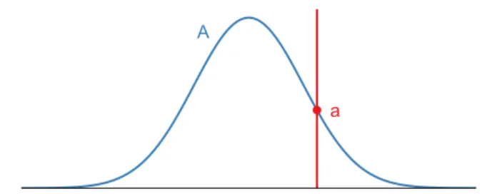
Figure 1.The probability distributionAquantifies potential errors. SamplingA produces a single pointa, introducing uncertainty, buta does not necessarily represent the true value. Many programs treataas the true value.
1.
Introduction
Applications that sense and reason about the complexity of the world use estimates. Mobile phone applications esti-mate location with GPS sensors, search estiesti-mates information needs from search terms, machine learning estimates hidden parameters from data, and approximate hardware estimates precise hardware to improve energy efficiency. The difference between an estimate and its true value isuncertainty. Every estimate has uncertainty due to random or systematic error. Random variables model uncertainty with probability distri-butions, which assign a probability to each possible value. For example, each flip of a biased coin may have a 90% chance of heads and 10% chance of tails. The outcome of one flip is only a sample and not a good estimate of the true value. Figure 1 shows a sample from a Gaussian distribution which is a poor approximation for the entire distribution.
Most programming languages force developers to reason about uncertain data with discrete types (floats, integers, and booleans). Motivated application developers reason about uncertainty in ad hoc ways, but because this task is complex, many more simply ignore uncertainty. For instance, we surveyed 100 popular smartphone applications that use GPS and find only one (Pizza Hut) reasons about the error in GPS measurements. Ignoring uncertainty creates three types of uncertainty bugswhich developers need help to avoid:
Using estimates as factsignores random noise in data and introduces errors.
Computation compounds errorssince computations on un-certain data often degrade accuracy significantly.
Conditionals ask boolean questionsof probabilistic data, leading to false positives and false negatives.
While probabilistic programming [6, 13, 15, 24, 25] and domain-specific solutions [1, 2, 11, 18, 28–30] address parts of this problem, they demand expertise far beyond what client applications require. For example in current probabilistic programming languages, domain experts create and query distributions through generative models. Current APIs for estimated data from these programs, sensors, big data, ma-chine learning, and other sources then project the resulting distributions into discrete types. We observe that the prob-abilistic nature of estimated data does not stop at the API boundary. Applications using estimated data are probabilistic programs too! Existing languages do not consider the needs of applications that consume estimated data, leaving their developers to face this difficult problem unaided.
This paper introduces theuncertain type,UncertainhTi, a programming language abstraction for arbitrary probability distributions. The syntax and semantics emphasize simplicity for non-experts. We describe how expert developers derive and expose probability distributions for estimated data. Simi-lar to probabilistic programming, the uncertain type defines an algebra over random variables to propagate uncertainty through calculations. We introduce a Bayesian network se-mantics for computations and conditional expressions. In-stead of eagerly evaluating probabilistic computations as in prior languages, we lazily evaluateevidencefor the condi-tions. Finally, we show how the uncertain type eases the use of prior knowledge to improve estimates.
Our novel implementation strategy performs lazy eval-uation by exploiting the semantics of conditionals. The UncertainhTiruntime creates a Bayesian network that rep-resents computations on distributions and then samples it at conditional expressions. A sample executes the computa-tions in the network. The runtime exploits hypothesis tests to take only as many samples as necessary for the particular conditional, rather than eagerly and exhaustively producing unnecessary precision (as in general inference over genera-tive models). These hypothesis tests both guarantee accuracy bounds and provide high performance.
We demonstrate these claims with three case studies. (1) We show howUncertainhTiimproves accuracy and ex-pressiveness of speed computations from GPS, a widely used hardware sensor. (2) We show howUncertainhTiexploits prior knowledge to minimize random noise in digital sensors. (3) We show howUncertainhTiencourages developers to explicitly reason about and improve accuracy in machine learning, using a neural network that approximates hard-ware [12, 26]. In concert, the syntax, semantics, and case studies illustrate thatUncertainhTieases probabilistic rea-soning, improves estimates, and helps domain experts and developers work with uncertain data.
Our contributions are (1) characterizing uncertainty bugs; (2)UncertainhTi, an abstraction and semantics for uncertain
data; (3) implementation strategies that make this semantics practical; and (4) case studies that show UncertainhTi’s potential to improve expressiveness and correctness.
2.
Motivation
Modern and emerging applications compute over uncertain data from mobile sensors, search, vision, medical trials, benchmarking, chemical simulations, and human surveys. Characterizing uncertainty in these data sources requires do-main expertise, but non-expert developers (perhaps with other expertise) are increasingly consuming the results. This sec-tion uses Global Posisec-tioning System (GPS) data to motivate a correct and accessible abstraction for uncertain data.
On mobile devices, GPS sensors estimate location. APIs for GPS typically include a position and estimated error radius (a confidence interval for location). The Windows Phone (WP) API returns three fields:
public double Latitude, Longitude; // location public double HorizontalAccuracy; // error estimate This interface encourages three types ofuncertainty bugs.
Interpreting Estimates as Facts Our survey of the top 100 WP and 100 Android applications finds 22% of WP and 40% of Android applications use GPS for location. Only 5% of the WP applications that use GPS read the error radius and only one application (Pizza Hut) acts on it. All others treat the GPS reading as a fact. Ignoring uncertainty this way causes errors such as walking through walls or driving on water.
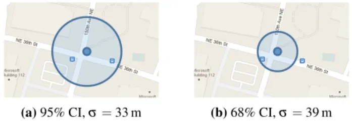
Current abstractions encourage this treatment by obscur-ing uncertainty. Consider the map applications on two differ-ent smartphone operating systems in Figure 2, which depict location with a point and horizontal accuracy as a circle. Smaller circlesshouldindicate less uncertainty, but the left larger circle is a 95% confidence interval (widely used for statistical confidence), whereas the right is a 68% confidence interval (one standard deviation of a Gaussian). The smaller circle has a higher standard deviation and is less accurate! (We reverse engineered this confidence interval detail.) A single accuracy number is insufficient to characterize the underlying error distribution or to compute on it. The hor-izontal accuracy abstraction obscures the true uncertainty, encouraging developers to ignore it completely.
Compounding Error Computation compounds uncertainty. To illustrate, we recorded GPS locations on WP while
walk-(a)95% CI,σ=33 m (b)68% CI,σ=39 m Figure 2.GPS samples at the same location on two smart-phone platforms. Although smaller circlesappearmore accu-rate, the WP sample in (a) is actually more accurate.
7 mph 59 mph
Usain Bolt
0 20 40 60
Time
Speed (mph)
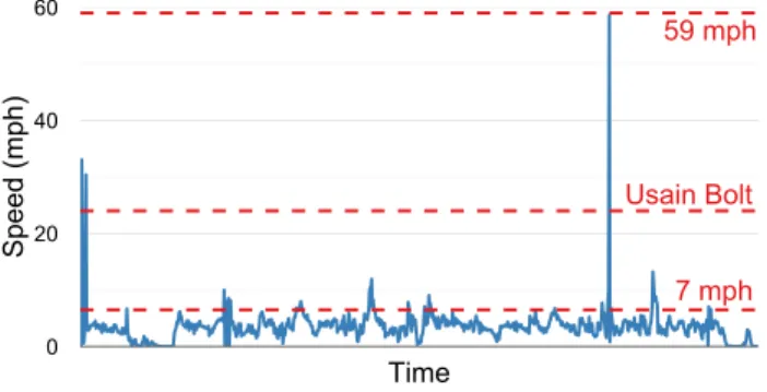
Figure 3.Speed computation on GPS data produces absurd walking speeds (59 mph, and 7 mph for 35 s, a running pace). ing and computed speed each second. Our inspection of smart-phone applications shows this computation on GPS data is very common. Figure 3 plots speed computed by the code in Figure 5(a) using the standard GPS API. Whereas Us-ain Bolt runs 100 m at 24 mph, the average human walks at 3 mph. This experimental data shows an average of 3.5 mph, 35 s spent above 7 mph (running speed), and absurd speeds of 30, 33, and 59 mph. These errors are significant in both magnitude and frequency. The cause is compounded error, since speed is a function oftwouncertain locations. When the locations have a 95% confidence interval of 4 m (the best that smartphone GPS delivers), speed has a 95% confidence interval of 12.7 mph. Current abstractions do not capture the compounding of error because they do not represent the dis-tribution nor propagate uncertainty through calculations.
Conditionals Programs eventually act on estimated data with conditionals. Consider using GPS to issue tickets for a 60 mph speed limit with the conditional Speed>60. If your actual speed is 57 mph and GPS accuracy is 4 m, this conditional gives a 32% probability of a ticket due to random noise alone. Figure 4 shows this probability across speeds and GPS accuracies. Boolean questions ignore the potential for random error, leading to false positives and negatives. Applications instead should ask probabilistic questions; for example, only issuing a ticket if the probability is very high that the user is speeding.
Without an appropriate abstraction for uncertain data, propagation of errors through computations, and prob-abilistic semantics for conditionals, correctness is out of reach for many developers.
3.
A First-Order Type for Uncertain Data
We propose a new generic data typeUncertainhTiand opera-tions to capture and manipulate uncertain data as probability distributions. The operations propagate distributions through computations and conditionals with an intuitive semantics that help developers program with uncertain data. The un-certain typeprogramming language abstraction is broadly applicable to many languages and we implemented proto-types in C#, C++, and Python. Unlike existing probabilistic
0% 25% 50% 75% 100%
56 58 60 62 64
Actual speed (mph)
Chance of speeding tick
et
GPS accuracy
1 m 2 m 4 m
Figure 4.Probability of issuing a speeding ticket at a 60 mph speed limit. With a true speed of 57 mph and GPS accuracy of 4 m, there is a 32% chance of issuing a ticket.
programming approaches, which focus on statistics and ma-chine learning experts,UncertainhTifocuses on creating an accessible interface for non-expert developers, who are in-creasingly encountering uncertain data.
This section first overviews UncertainhTi’s syntax and probabilistic semantics and presents an example. It then de-scribes the syntax and semantics for specifying distributions, computing with distributions by building a Bayesian network representation of computations, and executing conditional expressions by evaluating evidence for a conclusion. We then describe howUncertainhTimakes it easier for developers to improve estimates with domain knowledge. Section 4 de-scribes our lazy evaluation and sampling implementation strategies that make these semantics efficient.
Overview An object of typeUncertainhTiencapsulates a random variable of a numeric typeT. To represent computa-tions, the type’s overloaded operators constructBayesian net-works, directed acyclic graphs in which nodes represent ran-dom variables and edges represent conditional dependences between variables. The leaf nodes of these Bayesian networks are known distributions defined by expert developers. Inner nodes represent the sequence of operations that compute on these leaves. For example, the following code
Uncertain<double> a = new Gaussian(4, 1);
Uncertain<double> b = new Gaussian(5, 1);
Uncertain<double> c = a + b;
results in a simple Bayesian network +
a c
b
with two leaf nodes (shaded) and one inner node (white) rep-resenting the computationc = a + b.UncertainhTi evalu-ates this Bayesian network when it needs the distribution of
c, which depends on the distributions ofaandb. Here the distribution ofcis more uncertain thanaorb, as Figure 6 shows, since computation compounds uncertainty.
This paper describes a runtime that builds Bayesian net-works dynamically and then, much like a JIT, compiles those
double dt = 5.0; // seconds
GeoCoordinate L1 = GPS.GetLocation();
while (true) {
Sleep(dt); // wait for dt seconds GeoCoordinateL2 = GPS.GetLocation();
doubleDistance = GPS.Distance(L2, L1);
doubleSpeed = Distance / dt; print("Speed: " + Speed);
if(Speed > 4) GoodJob();
else SpeedUp();
L1 = L2; // Last Location = Current Location;
}
(a)Without the uncertain type
doubledt = 5.0; // seconds
Uncertain<GeoCoordinate> L1 = GPS.GetLocation();
while (true) {
Sleep(dt); // wait for dt seconds
Uncertain<GeoCoordinate> L2 = GPS.GetLocation();
Uncertain<double> Distance = GPS.Distance(L2, L1);
Uncertain<double> Speed = Distance / dt; print("Speed: " + Speed.E());
if (Speed > 4) GoodJob();
else if ((Speed < 4).Pr(0.9)) SpeedUp(); L1 = L2; // Last Location = Current Location;
}
(b)With the uncertain type
Figure 5.A simple fitness application (GPS-Walking), encouraging users to walk faster than 4 mph, implemented with and without the uncertain type. The typeGeoCoordinateis a pair ofdoubles (latitude and longitude) and so is numeric.
a b
c
Figure 6.The sumc=a+bis more uncertain thanaorb. expression trees to executable code at conditionals. The se-mantics establishes hypothesis tests at conditionals. The run-time samples by repeatedly executing the compiled code until the test is satisfied.
Example Program Figure 5 shows a simple fitness appli-cation (GPS-Walking) written in C#, both without (left) and with (right)UncertainhTi.GPS-Walkingencourages users to walk faster than 4 mph. TheUncertainhTiversion produces more accurate results in part because the type encourages the developer to reason about false positives and negatives. In particular, the developer chooses not to nag, admonishing users to SpeedUponly when it is very confident they are walking slowly. As in traditional languages,UncertainhTi only executes one side of conditional branches. Some proba-bilistic languages execute both sides of conditional branches to create probabilistic models, butUncertainhTimakes con-crete decisions at conditional branches, matching the host language semantics. We demonstrate the improved accuracy of theUncertainhTiversion ofGPS-Walkingin Section 5.1.
This example serves as a good pedagogical tool because of its simplicity, but the original embodies a real-world uncertainty problem becausemanysmartphone applications on all major platforms use the GPS API exactly this way. UncertainhTi’s simple syntax and semantics result in very few changes to the program: the developer only changes the variable types and the conditional operators.
3.1 Syntax with Operator Overloading
Table 1 shows the operators and methods ofUncertainhTi. UncertainhTidefines an algebra over random variables to propagate uncertainty through computations, overloading the usual arithmetic operators from the base numeric typeT.
Operators
Math (+− ∗/) op::UhTi →UhTi →UhTi Order (< >≤ ≥) op::UhTi →UhTi →UhBooli Logical (∧ ∨) op::UhBooli →UhBooli →UhBooli Unary (¬) op::UhBooli →UhBooli
Point-mass Pointmass::T→UhTi Conditionals
Explicit Pr::UhBooli →[0,1]→Bool Implicit Pr::UhBooli →Bool
Evaluation
Expected value E::UhTi →T
UhTiis shorthand forUncertainhTi.
Table 1.UncertainhTioperators and methods. Developers may override other types as well. Developers compute withUncertainhTias they would withT, and the Bayesian network the operators construct captures how error in an estimate flows through computations.
UncertainhTiaddresses two sources of random error: do-mainerror andapproximationerror. Domain error motivates our work and is the difference between an estimate and its true value. Approximation error is created becauseUncertainhTi must approximate distributions. Developers ultimately make concrete decisions on uncertain data through conditionals. UncertainhTi’s conditional operators enforce statistical tests at conditionals, mitigating both sources of error.
3.2 Identifying Distributions
The underlying probability distribution for uncertain data is specific to the problem domain. In many cases expert library developers already know these distributions, and sometimes they use them to produce crude error estimates such as the GPS horizontal accuracy discussed in Section 2. UncertainhTioffers these expert developers an abstraction to expose these distributions while preserving the simplic-ity of their current API. The non-expert developers who consume this uncertain data program against the common UncertainhTiAPI, which is very similar to the way they al-ready program with uncertain data today, but aids them in avoiding uncertainty bugs.
The expert developer has two broad approaches for select-ing the right distribution for their particular problem.
(1) Selecting a theoretical model. Many sources of uncer-tain data are amenable to theoretical models which library writers may adopt. For example, the error in the mean of a data set is approximately Gaussian by the Central Limit Theorem. Section 5.1 uses a theoretical approach for the
GPS-Walkingcase study.
(2) Deriving an empirical model. Some problems do not have or are not amenable to theoretical models. For these cases, expert developers may determine an error distribu-tion empirically by machine learning or other mechanisms. Section 5.3 uses an empirical approach for machine learning. Representing Distributions
There are a number of ways to store probability distributions. The most accurate mechanism stores the probability density function exactly. For finite domains, a simple map can as-sign a probability to each possible value [30]. For continuous domains, one might reason about the density function alge-braically [4]. For example, a Gaussian random variable with meanµand varianceσ2has density function
f(x) = 1 σ
√ 2π
exp
−(x−µ) 2
2σ2
.
An instance of a Gaussian random variable need only store this formula and values ofµandσ2to represent the variable
exactly (up to floating point error).
Exact representation has two major downsides. First, the algebra quickly becomes impractical under computation: even the sum of two distributions requires evaluating a con-volutedconvolution integral. Second, many important distri-butions for sensors, road maps, approximate hardware, and machine learning do not have closed-form density functions and so cannot be stored this way.
To overcome these issues,UncertainhTirepresents distri-butions through approximatesampling functions. Approxi-mation can be arbitrarily accurate given sufficient space and time [31], leading to an efficiency-accuracy trade-off. Many possible approximation schemes might be appropriate for UncertainhTi, including fixed vectors of random samples, Chebyshev polynomials [16], or sampling functions [23]. We use sampling functions because they implement a principled solution for balancing accuracy and efficiency.
3.3 Computing with Distributions
Developers combine uncertain data by using the usual opera-tors for arithmetic, logic, and comparison, andUncertainhTi manages the resultant uncertainty.UncertainhTioverloads such operators from the base typeTto work over distributions. For example, the example program in Figure 5(b) calculates the user’s speed by division:
Uncertain<double> Speed = Distance / dt;
D = A / B
E = D - C
-C /
E
B A
D
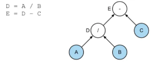
Figure 7. Bayesian network for a simple program with independent leaves.
The typeDoublehas a division operator of type /::Double→Double→Double.
The typeUncertainhDoubleilifts this operator to work over random variables, providing a new operator
/::UhDoublei →UhDoublei →UhDoublei. Note given xof type T, the semantics coercesx to type UncertainhTi with a pointmass distribution centered at x, so the denominatordt is cast to type UncertainhDoublei. The same lifting occurs on other arithmetic operators of type T →T →T, as well as comparison operators (typeT → T→Bool) and logical operators (typeBool→Bool→Bool). A lifted operator may have any type. For example, we can define real division of integers as typeInt→Int→Double, whichUncertainhTilifts without issue.
Instead of executing operations instantaneously, the lifted operators construct Bayesian network representations of the computations. A Bayesian network is a probabilistic graphical model and is a directed acyclic graph whose nodes represent random variables and whose edges represent conditional dependences between those variables [5]. Figure 7 shows an example of this Bayesian network representation. The shaded leaf nodes are known distributions (such as Gaussians) specified by expert developers, as previously noted. The final Bayesian network defines a joint distribution over all the variables involved in the computation:
Pr[A,B,C,D,E] =Pr[A]Pr[B]Pr[C]Pr[D|A,B]Pr[E|C,D]. The incoming edges to a node in the Bayesian network graph specify the other variables that the node’s variable depends on. For example,A has no dependences while Edepends on C and D. Since we know the distributions of the leaf nodesA,B, andC, we use the joint distribution to infer the marginal distributions of the variablesDandE, even though their distributions are not explicitly specified by the program. The conditional distributions of inner nodes are specified by their associated operators. For example, the distribution of Pr[D|A=a,B=b]in Figure 7 is simply a pointmass ata/b. Dependent Random Variables
Two random variablesXandYare independent if the value of one has no bearing on the value of the other.UncertainhTi’s Bayesian network representation assumes that leaf nodes are independent. This assumption is common in probabilistic pro-gramming, but expert developers can override it by specifying the joint distribution between two variables.
A = Y + X
B = A + X +
X +
B
X Y
A
(a)Wrong network
+
+ B
X Y
A
(b)Correct network Figure 8. Bayesian networks for a simple program with dependent leaves.
4 mph Pr[Speed > 4]
0 2 4 6 8 10
Speed (mph)
Figure 9.Uncertainty in data means there is only a probabil-itythatSpeed>4, not a concrete boolean value.
The UncertainhTi semantics automatically addresses program-induced dependences. For example, Figure 8(a) shows a simple program with a naive incorrect construc-tion of its Bayesian network. This network implies that the operands to the addition that definesBare independent, but in fact both operands depend on the same variableX. When producing a Bayesian network, UncertainhTi’s operators echo static single assignment by determining that the two
Xoccurrences refer to the same value, and soAdepends on the sameXasB. Our analysis produces the correct Bayesian network in Figure 8(b). Because the Bayesian network is constructed dynamically and incrementally during program execution, the resulting graph remains acyclic.
3.4 Asking the Right Questions
After computing with uncertain data, programs use it in conditional expressions to make decisions. The example program in Figure 5 compares the user’s speed to 4 mph. Of course, since speed is computed with uncertain estimates of location, it too is uncertain. The naive conditionalSpeed>4 incorrectly asks a deterministic question of probabilistic data, creating uncertainty bugs described in Section 2.
UncertainhTidefines the semantics of conditional expres-sions involving uncertain data by computingevidencefor a conclusion. This semantics encourages developers to ask ap-propriate questions of probabilistic data. Rather than asking “is the user’s speed faster than 4 mph?”UncertainhTiasks “how much evidence is there that the user’s speed is faster than 4 mph?” The evidence that the user’s speed is faster than 4 mph is the quantity Pr[Speed>4]; in Figure 9, this is the area under the distribution of the variableSpeedto the right
of 4 mph. Since we are considering probability distributions, the areaAsatisfies 0≤A≤1.
When the developer writes a conditional expression if(Speed > 4) ...
the program applies the lifted version of the>operator >::UncertainhTi →UncertainhTi →UncertainhBooli. This operator creates a Bernoulli distribution with param-eter p∈[0,1], which by definition is the probability that Speed>4 (i.e., the shaded area under the curve). Unlike other probabilistic programming languages,UncertainhTi executes only a single branch of the conditional to match the host language’s semantics. TheUncertainhTiruntime must therefore convert this Bernoulli distribution to a concrete boolean value. This conditional uses the implicit conditional operator, which compares the parameterpof the Bernoulli distribution to 0.5, asking whether the Bernoulli is more likely than not to be true. This conditional therefore evaluates whether Pr[Speed>4]>0.5, asking whether it is more likely that the user’s speed is faster than 4 mph.
Using an explicit conditional operator, developers may specify a threshold to compare against. The second compari-son in Figure 5(b) uses this explicit operator:
else if ((Speed < 4).Pr(0.9)) ...
This conditional evaluates whether Pr[Speed<4]>0.9. The power of this formulation is reasoning about false positives and negatives. Even if the mean of the distribution is on one side of the conditional threshold, the distribution may be very wide, so there is still a strong likelihood that the opposite conclusion is correct. Higher thresholds for the explicit operator require stronger evidence, and produce fewer false positives (extra reports when ground truth is false) but more false negatives (missed reports when ground truth is true). In this case, the developer chooses to favor some false positives for encouraging users (GoodJob), and to limit false positives when admonishing users (SpeedUp) by demanding stronger evidence that they are walking slower than 4 mph. Hypothesis Testing for Approximation Error
BecauseUncertainhTiapproximates distributions, we must consider approximation error in conditional expressions. We use statistical hypothesis tests, which make inferences about population statistics based on sampled data.UncertainhTi establishes a hypothesis test when evaluating the implicit and explicit conditional operators. In the implicit case above, the null hypothesis isH0: Pr[Speed>4]≤0.5 and the alternate hypothesisHA: Pr[Speed>4]>0.5. Section 4.3 describes
our sampling process for evaluating these tests in detail. Hypothesis tests introduce a ternary logic. For example, given the code sequence
if(A < B) ...
else if (A >= B) ...
neither branch may be true because the runtime may not be able to reject the null hypothesis for either conditional at the required confidence level. This behavior is not new: just
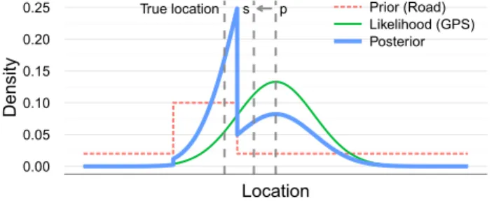
s p True location
0.00 0.05 0.10 0.15 0.20 0.25
Location
Density
Prior (Road) Likelihood (GPS) Posterior
Figure 10. Domain knowledge as a prior distribution im-proves the quality of GPS estimates.
as programs should not compare floating point numbers for equality, neither should they compare distributions for equal-ity. However, for problems thatrequirea total order, such as sorting algorithms,UncertainhTiprovides the expected value operatorE. This operator outputs an element of typeT and so it preserves the base type’s ordering properties. 3.5 Improving Estimates
Bayesian statistics represents the state of the world with degrees of belief and is a powerful mechanism for improving the quality of estimated data. Given two random variables,B representing the target variable to estimate (e.g., the user’s location), andEthe estimation process (e.g., the GPS sensor output), Bayes’ theorem says that
Pr[B=b|E=e] =Pr[E=e|B=b]·Pr[B=b]
Pr[E=e] .
Bayes’ theorem combines evidence from estimation pro-cesses (the valueeofE) with hypotheses about the true value bof the target variableB. We call Pr[B=b]theprior distri-bution, our belief aboutBbefore observing any evidence, and Pr[B=b|E=e]theposteriordistribution, our belief aboutB after observing evidence.
UncertainhTiunlocks Bayesian statistics by encapsulating entire data distributions. Abstractions that capture only single point estimates are insufficient for this purpose and force developers to resort to ad-hoc heuristics to improve estimates. Incorporating Knowledge with Priors
Bayesian inference is powerful because developers can en-code their domain knowledge as prior distributions, and use that knowledge to improve the quality of estimates. For ex-ample, a developer working with GPS can provide a prior distribution that assigns high probabilities to roads and lower probabilities elsewhere. This prior distribution achieves a “road-snapping” behavior [21], fixing the user’s location to nearby roads unless GPS evidence to the contrary is very strong. Figure 10 illustrates this example – the mean shifts fromptos, closer to the road the user is actually on.
Specifying priors, however, requires a knowledge of statis-tics beyond the scope of most developers. In our current im-plementation, applications specify domain knowledge with constraint abstractions. Expert developers add preset prior distributions to their libraries for common cases. For example,
GPS libraries would include priors for driving (e.g., roads and driving speeds), walking (walking speeds), and being on land. Developers combine priors through flags that select constraints specific to their application. The library applies the selected priors, improving the quality of estimates with-out much burden on developers. This approach is not very satisfying because it is not compositional, so the application cannot easily mix and match priors from different sources (e.g., maps, calendars, and physics for GPS). We anticipate future work creating an accessible and compositional abstrac-tion for prior distribuabstrac-tions, perhaps with the Bayes operator P]Qfor sampled distributions by Park et al. [23].
4.
Implementation
This section describes our practical and efficient C# imple-mentation of theUncertainhTiabstraction. We also imple-mented prototypes ofUncertainhTiin C++ and Python and believe most high-level languages could easily implement it. 4.1 Identifying Distributions
UncertainhTiapproximates distributions withsampling func-tions, rather than storing them exactly, to achieve expressive-ness and efficiency. A sampling function has no arguments and returns a new random sample, drawn from the distribu-tion, on each invocation [23]. For example, a pseudo-random number generator is a sampling function for the uniform dis-tribution, and the Box-Mueller transform [8] is a sampling function for the Gaussian distribution.
In theGPS-Walkingapplication in Figure 5(b), the variables
L1andL2are distributions obtained from the GPS library. The expert developer who implements the GPS library derives the correct distribution and provides it toUncertainhTias a sampling function. Bornholt [7] shows in detail the derivation for the error distribution of GPS data. The resulting model says that the posterior distribution for a GPS estimate is
Pr[Location=p|GPS=Sample] =Rayleigh(kSample−pk;ε/
√ ln 400)
whereSampleis the raw GPS sample from the sensor,εis the sensor’s estimate of the 95% confidence interval for the location (i.e., the horizontal accuracy from Section 2), and the Rayleigh distribution [22] is a continuous non-negative single-parameter distribution with density function
Rayleigh(x;ρ) = x ρ2exp
− x 2
2ρ2
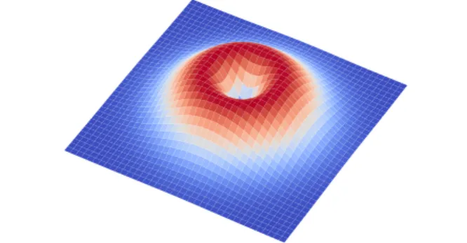
, x≥0. Figure 11 shows the posterior distribution given a particular value ofε. Most existing GPS libraries return a coordinate (the center of the distribution) and presentεas a confidence parameter most developers ignore. Figure 11 shows that the true location isunlikelyto be in the center of the distribution and more likely to be some fixed radius from the center.
We built a GPS library that captures error in its estimate withUncertainhTiusing this distribution. Figure 12 shows our library functionGPS.GetLocation, which returns an instance ofUncertainhGeoCoordinateiby implementing a
Figure 11.The posterior distribution for GPS is a distribution over the Earth’s surface.
Uncertain<GeoCoordinate> GetLocation() {
// Get the estimates from the hardware
GeoCoordinate Point = GPS.GetHardwareLocation();
double Accuracy = GPS.GetHardwareAccuracy();
// Compute epsilon
double epsilon = Accuracy / Math.Sqrt(Math.Log(400));
// Define the sampling function
Func<GeoCoordinate> SamplingFunction = () => {
double radius, angle, x, y;
// Samples the distribution in Figure 11 using // polar coordinates
radius = Math.RandomRayleigh(epsilon); angle = Math.RandomUniform(0, 2*Math.PI);
// Convert to x,y coordinates in degrees
x = Point.Longitude;
x += radius*Math.Cos(angle)*DEGREES_PER_METER; y = Point.Latitude;
y += radius*Math.Sin(angle)*DEGREES_PER_METER;
// Return the GeoCoordinate return new GeoCoordinate(x, y); }
// Return the instance of Uncertain<T>
return new Uncertain<GeoCoordinate>(SamplingFunction); }
Figure 12.TheUncertainhTiversion ofGPS.GetLocation
returns an instance ofUncertainhGeoCoordinatei.
sampling function to draw samples from the posterior distri-bution. The sampling function captures the values ofPoint
andAccuracy. Although the sampling function is later in-voked many times to draw samples from the distribution, the GPS hardware functionsGetHardwareLocationand
GetHardwareAccuracyare only invoked once for each call toGetLocation.
4.2 Computing with Distributions
UncertainhTipropagates error through computations by over-loading operators from the base typeT. These lifted operators dynamically construct Bayesian network representations of the computations they represent as the program executes. However, an alternate implementation could statically build a Bayesian network and only dynamically perform hypothesis tests at conditionals. We use the Bayesian network to define the sampling function for a computed variable in terms of the sampling functions of its operands. We only evaluate the sampling function at conditionals and so the root node of a network being sampled is always a comparison operator.
The computed sampling function uses the standard ances-tral samplingtechnique for graphical models [5]. Because
the Bayesian network is directed and acyclic, its nodes can be topologically ordered. We draw samples in this topological order, starting with each leaf node, for which sampling func-tions are explicitly defined. These samples then propagate up the Bayesian network. Each inner node is associated with an operator from the base type, and the node’s children have already been sampled due to the topological order, so we simply apply the base operator to the operand samples to generate a sample from an inner node. This process continues up the network until reaching the root node of the network, generating a sample from the computed variable. The topo-logical order guarantees that each node is visited exactly once in this process, and so the sampling process terminates.
In theGPS-Walkingapplication in Figure 5(b), the user’s speed is calculated by the line
Uncertain<double> Speed = Distance / dt;
The lifted division operator constructs a Bayesian network for this computation:
/
Distance Speed
dt
t d
Here shaded nodes indicate leaf distributions, for which sampling functions are defined explicitly.
To draw a sample from the variable Speed, we draw a sample from each leaf: a sampledfromDistance(defined by the GPS library) andtfromdt(a pointmass distribution, so all samples are equal). These samples propagate up the network to theSpeednode. Because this node is a division operator, the resulting sample fromSpeedis simplyd/t. 4.3 Asking Questions with Hypothesis Tests
UncertainhTi’s conditional and evaluation operators address the domain error that motivates our work. These operators require concrete decisions under uncertainty. The conditional operators must select one branch target to execute. In the GPS-Walkingapplication in Figure 5(b), a conditional operator
if(Speed > 4)...
must decide whether or not to enter this branch. Sec-tion 3.4 describes howUncertainhTi executes this condi-tional by comparing the probability Pr[Speed>4]to a de-fault threshold 0.5, asking whether it is more likely than not that Speed>4. To control approximation error, this comparison is performed by a hypothesis test, with null hy-pothesisH0: Pr[Speed>4]≤0.5 and alternate hypothesis HA: Pr[Speed>4]>0.5.
Sampling functions in combination with this hypothesis test control the efficiency-accuracy trade-off that approxima-tion introduces. A higher confidence level for the hypothesis test leads to fewer approximation errors but requires more samples to evaluate. We perform the hypothesis test using Wald’ssequential probability ratio test(SPRT) [32] to dy-namically choose the right sample size for a particular
condi-tional, only taking as many samples as necessary to obtain a statistically significant result.
We specify a step size, sayk=10, and start by drawing n=ksamples from the Bernoulli distribution Speed>4. We then apply the SPRT to these samples to decide if the parameter p of the distribution (i.e., the probability Pr[Speed>4]) is significantly different from 0.5. If so, we can terminate immediately and take (or not take) the branch, depending on in which direction the significance lies. If the result is not significant, we draw another batch ofksamples, and repeat the process with the nown=2kcollection of samples. We repeat this process until either a significant result is achieved or a maximum sample size is reached to ensure termination. The SPRT ensures that this repeated sampling and testing process still achieves overall bounds on the probabilities of false positives (significance level) and false negatives (power).
Sampling functions and a Bayesian network representa-tion may draw as many samples as we wish from any given variable. We may therefore exploit sequential methods, such as the SPRT, which do not fix the sample size for a hypothesis test in advance. Sequential methods are a principled solution to the efficiency-accuracy trade-off. They ensure we draw the minimum necessary number of samples for a sufficiently ac-curate result for each specific conditional. This goal-oriented sampling approach is a significant advance over previous ran-dom sampling approaches, which compute with a fixed pool of samples. These approaches do not efficiently control the effect of approximation error.
Wald’s SPRT is optimal in terms of average sample size, but is potentially unbounded in any particular instance, so termination is not guaranteed. The artificial maximum sample size we introduce to guarantee termination has a small effect on the actual significance level and power of the test. We anticipate adapting the considerable body of work on group sequential methods [17], widely used in medical clinical trials, which provide “closed” sequential hypothesis tests with guaranteed upper bounds on the sample size.
We cannot apply the same sequential testing approach to the evaluation operatorE, since there are no alternatives to compare against (i.e., no goal to achieve). Currently for this operator we simply draw a fixed number of samples and return their mean. We believe a more intelligent adaptive sampling process, sampling until the mean converges, may improve the performance of this approach.
5.
Case Studies
We use three case studies to explore the expressiveness and correctness ofUncertainhTion uncertain data. (1) We show howUncertainhTiimproves accuracy and expressiveness of speed computations from GPS, a widely used hardware sen-sor. (2) We show howUncertainhTiexploits prior knowledge to minimize random noise in digital sensors. (3) We show howUncertainhTiencourages developers to explicitly
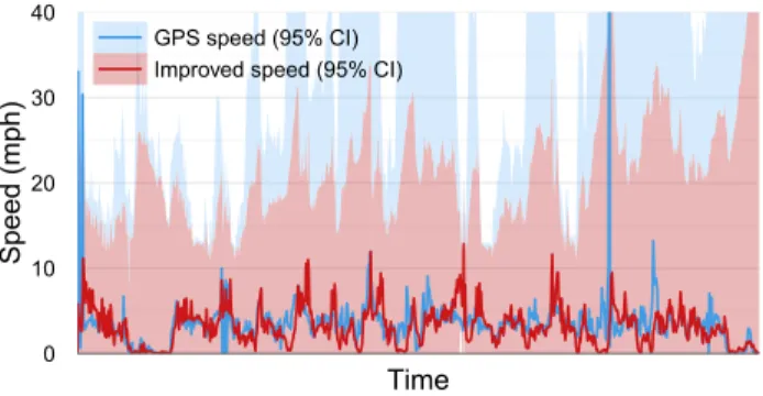
rea-0 10 20 30 40
Time
Speed (mph)
GPS speed (95% CI) Improved speed (95% CI)
Figure 13.Data from theGPS-Walkingapplication. Develop-ers improve accuracy with priors and remove absurd values. son about and improve accuracy in machine learning, using a neural network that approximates hardware [12, 26]. 5.1 Uncertain<T>on Smartphones: GPS-Walking The modern smartphone contains a plethora of hardware sen-sors. Thousands of applications use the GPS sensor, and many compute distance and speed from GPS readings. Our walking speed case study serves double duty, showing how uncer-tainty bugs occur in practice as well as a clear pedagogical demonstration of howUncertainhTiimproves correctness and expressiveness. We wrap the Windows Phone (WP) GPS location services API withUncertainhTi, exposing the error distribution. TheGPS-Walkingapplication estimates the user’s speed by taking two samples from the GPS and computing the distance and time between them. Figure 5 compares the code forGPS-Walkingwith and without the uncertain type.
Defining the Distributions OurUncertainhTiGPS library provides the function
Uncertain<GeoCoordinate> GPS.GetLocation();
which returns a distribution over the user’s possible locations. Section 4.1 overviews how to derive the GPS distribution, and Figure 12 shows the implementation.
Computing with Distributions GPS-Walkinguses locations from the GPS library to calculate the user’s speed, since Speed=∆Distance/∆Time. Of course, since the locations are estimates, so too is speed. The developer must change the line
print("Speed: " + Speed);
from the original program in Figure 5(a), sinceSpeednow has typeUncertainhDoublei. It now prints the expected value
Speed.E()of the speed distribution.
We testedGPS-Walkingby walking outside for 15 minutes. Figure 13 shows the expected valuesSpeed.E()measured each second by the application (GPS speed). The uncertainty of the speed calculation, with extremely wide confidence intervals, explains the absurd values.
Conditionals GPS-Walkingencourages users to walk faster than 4 mph with messages triggered by conditionals. The original implementation in Figure 5(a) uses naive condition-als, which are susceptible to random error. For example, on
our test data, such conditionals would report the user to be walking faster than 7 mph (a running pace) for 30 seconds.
TheUncertainhTiversion ofGPS-Walkingin Figure 5(b) evaluates evidence to execute conditionals. The conditional
if(Speed > 4) GoodJob();
asks if it ismore likely than notthat the user is walking fast. The second conditional
else if ((Speed < 4).Pr(0.9)) SpeedUp();
asks if there is at least a 90% chance the user is walking slowly. This requirement is stricter than the first conditional because we do not want to unfairly admonish the user (i.e., we want to avoid false positives). Even the simplermore likely than notconditional improves the accuracy ofGPS-Walking: such a conditional would only report the user as walking faster than 7 mph for 4 seconds.
Improving GPS Estimates with Priors Because GPS-WalkingusesUncertainhTi, we may incorporate prior knowl-edge to improve the quality of its estimates. Assume for simplicity that users only invokeGPS-Walkingwhen walking. Since humans are incredibly unlikely to walk at 60 mph or even 10 mph, we specify a prior distribution over likely walk-ing speeds. Figure 13 shows the improved results (Improved speed). The confidence interval for the improved data is much tighter, and the prior knowledge removes the absurd results, such as walking at 59 mph.
Summary Developers need only make minimal changes to the originalGPS-Walking application and are rewarded with improved correctness. They improve accuracy by rea-soning correctly about uncertainty and eliminating absurd data with domain knowledge. This complex logic is difficult to implement without the uncertain type because a developer must know the error distribution for GPS, how to propagate it through calculations, and how to incorporate domain knowl-edge to improve the results. The uncertain type abstraction hides this complexity, improving programming productivity and application correctness.
5.2 Uncertain<T>with Sensor Error: SensorLife This case study emulates a binary sensor with Gaussian noise to explore accuracy when ground truth is available. For many problems using uncertain data, ground truth is difficult and costly to obtain, but it is readily available in this problem formulation. This case study shows howUncertainhTimakes it easier for non-expert developers to work with noisy sensors. Furthermore, it shows how expert developers can simply and succinctly use domain knowledge (i.e., the fact that the noise is Gaussian with known variance) to improve these estimates. We use Conway’s Game of Life, a cellular automaton that operates on a two-dimensional grid of cells that are each dead or alive. The game is broken up into generations. During each generation, the program updates each cell by (i) sensing the state of the cell’s 8 neighbors, (ii) summing the binary value (dead or alive) of the 8 neighbors, and (iii) applying the following rules to the sum:
1. A live cell with 2 or 3 live neighbors lives. 2. A live cell with less than 2 live neighbors dies. 3. A live cell with more than 3 live neighbors dies. 4. A dead cell with exactly 3 live neighbors becomes live. These rules simulate survival, underpopulation, overcrowd-ing, and reproduction, respectively. Despite simple rules, the Game of Life provides complex and interesting dynamics (e.g., it is Turing complete [3]). We focus on the accuracy of sensing if the neighbors are dead or alive.
Defining the Distributions The original Game of Life’s discrete perfect sensors define our ground truth. We view each cell as being equipped with up to eight sensors, one for each of its neighbors. Cells on corners and edges of the grid have fewer sensors. Each perfect sensor returns a binary values∈ {0,1}indicating if the associated neighbor is alive. We artificially induce zero-mean Gaussian noiseN(0,σ)
on each of these sensors, whereσ is the amplitude of the
noise. Each sensor now returns a real number, not a binary value. We define three versions of this noisy Game of Life: NaiveLifereads a single sample from each noisy sensor and
sums the results directly to count the live neighbors. SensorLifewraps each sensor withUncertainhTi. The sum
uses the overloaded addition operator and each sensor may be sampled multiple times in a single generation. BayesLifeuses domain knowledge to improveSensorLife, as
we describe below.
Our construction results in some negative sensor readings, but choosing a non-negative noise distribution, such as the Beta distribution, does not appreciably change our results.
Computing with Distributions Errors in each sensor are independent, so the function that counts a cell’s live neighbors is almost unchanged:
Uncertain<double> CountLiveNeighbors(Cell me) {
Uncertain<double> sum = new Uncertain<double>(0.0);
foreach (Cell neighbor in me.GetNeighbors()) sum = sum + SenseNeighbor(me, neighbor);
return sum; }
Because each sensor now returns a real number rather than a binary value, the count of live neighbors is now a distri-bution over real numbers rather than an integer. Operator overloading means that no further changes are necessary, as the addition operator will automatically propagate uncertainty into the resulting sum.
Conditionals The Game of Life applies its rules with four conditionals to the output ofCountLiveNeighbors:
bool IsAlive = IsCellAlive(me);
bool WillBeAlive = IsAlive;
Uncertain<double> NumLive = CountLiveNeighbors(me);
if (IsAlive && NumLive < 2) WillBeAlive = false;
else if (IsAlive && 2 <= NumLive && NumLive <= 3) WillBeAlive = true;
else if (IsAlive && NumLive > 3) WillBeAlive = false;
else if (!IsAlive && NumLive == 3) WillBeAlive = true;
Each comparison involvingNumLiveimplicitly performs a hypothesis test.
0 2 4 6 8
0.0 0.1 0.2 0.3
Noise amplitude (sigma)
Incorrect decisions (%)
NaiveLife SensorLife BayesLife
(a)Rate of incorrect decisions
0 50 100 150
0.0 0.1 0.2 0.3
Noise amplitude (sigma)
Samples per choice
NaiveLife SensorLife BayesLife
(b)Samples required for each cell
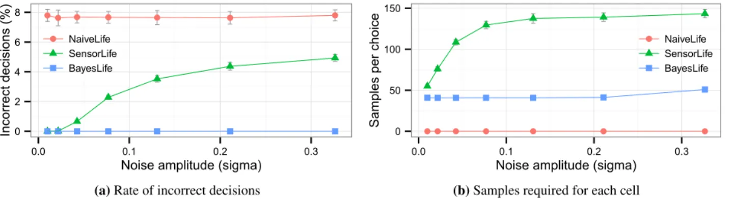
Figure 14.SensorLifeusesUncertainhTito significantly decrease the rate of incorrect decisions compared to a naive version, but requires more samples to make decisions.BayesLifeincorporates domain knowledge intoSensorLifefor even better results.
Evaluation We compare the noisy versions of the Game of Life to the precise version. We perform this comparison across a range of noise amplitude valuesσ. Each execution
randomly initializes a 20×20 cell board and performs 25 generations, evaluating a total of 10000 cell updates. For each noise levelσ, we execute each Game of Life 50 times. We
report means and 95% confidence intervals.
Figure 14(a) shows the rate of incorrect decisions (y-axis) made by each noisy Game of Life at various noise levels (x-axis).NaiveLifehas a consistent error rate of 8%, as it takes only a small amount of noise to cross the integer thresholds in the rules of the Game of Life.SensorLife’s errors scale with noise, as it considers multiple samples and so can correct smaller amounts of noise. At all noise levels,SensorLifeis considerably more accurate thanNaiveLife.
Mitigating noise has a cost, asUncertainhTimust sample each sensor multiple times to evaluate each conditional. Figure 14(b) shows the number of samples drawn for each cell update (y-axis) by each noisy Game of Life at various noise levels (x-axis). ClearlyNaiveLifeonly draws one sample per conditional. The number of samples forSensorLifeincreases as the noise level increases, because noisier sensors require more computation to reach a conclusion at the conditional.
Improving Estimates SensorLifeachieves better results than
NaiveLifedespite not demonstrating any knowledge of the fact that the underlying true state of a sensor must be either 0 or 1. To improveSensorLife, an expert can exploit knowledge of the distribution and variance of the sensor noise. We call this improved versionBayesLife.
Letvbe the raw, noisy sensor reading, andsthe underlying true state (either 0 or 1). Thenv=s+N(0,σ)for someσwe know. Sincesis binary, we have twohypothesesfors:H0says s=0 andH1sayss=1. The raw sensor readingvis evidence, and Bayes’ theorem calculates aposterior probability
Pr[H0|v] =Pr[v|H0]Pr[H0]/Pr[v]
forH0given the evidence, and similarly forH1. To improve an estimate, we calculate which ofH0andH1is more likely under the posterior probability, and fix the sensor reading to be 0 or 1 accordingly.
This formulation requires (i) the prior likelihoods Pr[H0] and Pr[H1]; and (ii) a likelihood function to calculate Pr[v|H0]
and Pr[v|H1]. We assume no prior knowledge, so bothH0and H1 are equally likely: Pr[H0] =Pr[H1] =0.5. Because we know the noise is Gaussian, we know the likelihood function is just the likelihood thatN(0,σ) =s−vfor each ofs=0
and 1, which we calculate trivially using the Gaussian density function. We need not calculate Pr[v]since it is a common denominator of the two probabilities we compare.
To implementBayesLifewe wrap each sensor with a new functionSenseNeighborFixed. Since the two likelihoods Pr[v|H0]and Pr[v|H1]have the same variance and shape and are symmetric around 0 and 1, respectively, and the priors are equal, the hypothesis with higher posterior probability is simply the closer of 0 or 1 tov. The implementation is therefore trivial:
Uncertain<double>
SenseNeighborFixed(Cell me, Cell neighbor) {
Func<double> samplingFunction = () => {
Uncertain<double> Raw = SenseNeighbor(me, neighbor);
double Sample = Raw.Sample();
return Sample > 0.5 ? 1.0 : 0.0; };
return new Uncertain<double>(samplingFunction); }
Evaluation of BayesLife Figure 14(a) shows thatBayesLife
makes no mistakes at all at these noise levels. At noise levels higher thanσ=0.4, considering individual samples in iso-lation breaks down as the values become almost completely random. A better implementation could calculate joint like-lihoods with multiple samples, since each sample is drawn from the same underlying distribution. Figure 14(b) shows thatBayesLiferequires fewer samples thanSensorLife, but of course still requires more samples thanNaiveLife.
5.3 Uncertain<T>for Machine Learning: Parakeet This section explores usingUncertainhTifor machine learn-ing, inspired byParrot[12], which trains neural networks for approximate hardware. We study the Sobel operator from the Parrot evaluation, which calculates the gradient of im-age intensity at a pixel. Parrot creates a neural network that approximates the Sobel operator.
Machine learning algorithms estimate the true value of a function. One source of uncertainty in their estimates is generalization error, where predictions are good on training data but poor on unseen data. To combat this error, Bayesian machine learning considers distributionsof estimates, re-flecting how different estimators would answer an unseen input. Figure 15 shows for one such input a distribution of neural network outputs created by the Monte Carlo method described below, the output from the single naive neural net-work Parrot trains, and the true output. The one Parrot value is significantly different from the correct value. Using a dis-tribution helps mitigate generalization error by recognizing other possible predictions.
Computation amplifies generalization error. For example, edge-detection algorithms use the Sobel operator to report an edge if the gradient is large (e.g.,s(p)>0.1). Though Parrot approximates the Sobel operator well, with an average root-mean-square error of 3.4%, using its output in such a conditional is a computation. This computation amplifies the error and results in a 36% false positive rate. In Figure 15, by considering the entire distribution, the evidence for the conditions(p)>0.1 is only 70%. To accurately consume estimates, developers must consider the effect of uncertainty not just on direct output but on computations that consume it. We introduceParakeet, which approximates code using Bayesian neural networks, and encapsulates the distribution withUncertainhTi. This abstraction encourages developers to consider uncertainty in the machine learning prediction. We evaluateParakeetby approximating the Sobel operators(p)
and computing the edge detection conditionals(p)>0.1.
Identifying the Distribution We seek aposterior predictive distribution(PPD), which tells us for a given input how likely each possible output is to be correct, based on the training data. Intuitively, this distribution reflects predictions from otherneural networks that also explain the training data well. Formally, a neural network is a function y(x;w) that approximates the output of a target functionf(x). The weight vectorwdescribes how each neuron in the network relates to the others. Traditional training uses example inputs and outputs to learn a single weight vectorwfor prediction. In a Bayesian formulation, we learn the PPD p(t|x,D) (the distribution in Figure 15), a distribution of predictions of
f(x)given the training dataD.
We adopt the hybrid Monte Carlo algorithm to create samples from the PPD [20]. Each sample describes a neural network. Intuitively, we create multiple neural networks by perturbing the search. Formally, we sample the posterior distributionp(w|D)to approximate the PPDp(t|x,D)using Monte Carlo integration, since
p(t|x,D) =
Z
p(t|x,w)p(w|D)dw.
The instance ofUncertainhTi thatParakeet returns draws samples from this PPD. Each sample ofp(w|D)from hybrid Monte Carlo is a vectorwof weights for a neural network.
True value s(p) > 0.1 Parrot value
0.00 0.05 0.10 0.15 0.20
Value of Sobel operator, s(p)
Probability
Figure 15. Error distribution for Sobel approximated by neural networks. Parrot experiences a false positive on this test, whichParakeeteliminates by evaluating theevidence thats(p)>0.1 (the shaded area).
To evaluate a sample from the PPDp(t|x,D), we execute a neural network using the weightswand inputx. The resulting output is a sample of the PPD.
We execute hybrid Monte Carlo offline and capture a fixed number of samples in a training phase. We use these samples at runtime as a fixed pool for the sampling function. If the sample size is sufficiently large, this approach approximates true sampling well. As with other Markov chain Monte Carlo algorithms, the next sample in hybrid Monte Carlo depends on the current sample, which improves on pure random walk behavior that scales poorly in high dimensions. To compensate for this dependence we discard most samples and only retain everyMthsample for some largeM.
Hybrid Monte Carlo has two downsides. First, we must execute multiple neural networks (one for each sample of the PPD). Second, it often requires hand tuning to achieve practical rejection rates. Other PPD approximations strike dif-ferent trade-offs. For example, a Gaussian approximation [5] to the PPD would mitigate all these downsides, but may be an inappropriate approximation in some cases. Since the Sobel operator’s posterior is approximately Gaussian (Figure 15), a Gaussian approximation may be appropriate.
Evaluation We approximate the Sobel operator with Para-keet, using 5000 examples for training and a separate 500 examples for evaluation. For each evaluation example we compute the ground truth s(p)>0.1 and then evaluate this conditional using UncertainhTi, which asks whether Pr[s(p)>0.1]>αfor varying thresholdsα.
Figure 16 shows the results of our evaluation. Thex-axis plots a range of conditional thresholdsα and they-axis plots precision and recall for the evaluation data. Precision is the probability that a detected edge is actually an edge, and so de-scribes false positives. Recall is the probability that an actual edge is detected, and so describes false negatives. Because Parrot does not consider uncertainty, it locks developers into a particular balance of precision and recall. In this example, Parrot provides 100% recall, detecting all actual edges, but only 64% precision, so 36% of reported edges are false pos-itives. With a conditional threshold, developers select their own balance. For example, a threshold ofα=0.8 (i.e.,
eval-Parrot Precision Parrot Recall
60 80 100
0.5 0.6 0.7 0.8 0.9
Conditional threshold
Precision/Recall (%)
Parakeet
Precision Recall
Figure 16.Developers choose a balance between false posi-tives and negaposi-tives withParakeetusingUncertainhTi. uating Pr[s(p)>0.1]>0.8) results in 71% recall and 99% precision, meaning more false negatives (missed edges) but fewer false positives. The ideal balance of false positives and negatives depends on the particular application and is now in the hands of the developer.
Summary Machine learning approximates functions and so introduces uncertainty. Failing to consider uncertainty causes uncertainty bugs; even though Parrot approximates the Sobel operator with 3.4% average error, using this approximation in a conditional results in a 36% false positive rate.Parakeetuses UncertainhTi, which encourages the developer to consider the effect of uncertainty on machine learning predictions. The results onParakeetshow that developers may easily con-trol the balance between false positives and false negatives, as appropriate for the application, usingUncertainhTi. Of course,UncertainhTiis not a panacea for machine learning. Our formulation leverages a probabilistic interpretation of neural networks, which not all machine learning techniques have, and only addresses generalization error.
These case studies highlight the need for a programming language solution for uncertainty. Many systems view error in a local scope, measuring its effect only on direct output, but as all the case studies clearly illustrate, the effect of uncertainty on programs is inevitably global. We cannot view estimation processes such as GPS and machine learning in isolation. UncertainhTi encourages developers to reason about how local errors impact the entirety of their programs.
6.
Related Work
This section relates our work to programming languages with statistical semantics or that support solving statistical problems. Because we use, rather than add to, the statistics literature, prior sections cite this literature as appropriate.
Probabilistic Programming Prior work has focused on the needs of experts. Probabilistic programming creates genera-tive models of problems involving uncertainty by introducing random variables into the syntax and semantics of a program-ming language. Experts encode generative models which the program queries through inference techniques. The founda-tion of probabilistic programming is the monadic structure of
earthquake = Bernoulli(0.0001) burglary = Bernoulli(0.001) alarm = earthquake or burglary
if(earthquake)
phoneWorking = Bernoulli(0.7)
else
phoneWorking = Bernoulli(0.99)
observe(alarm) # If the alarm goes off...
query(phoneWorking) # ...does the phone still work?
Figure 17.A probabilistic program. To infer the probability ofphoneWorkingrequires exploring both branches [10].
probability distributions [14, 25], an elegant representation of joint probability distributions (i.e., generative models) in a functional language. Researchers have evolved this idea into a variety of languages such as BUGS [13], Church [15], Fun [6], and IBAL [24].
Figure 17 shows an example probabilistic program that infers the likelihood that a phone is working given that an alarm goes off. The program queries the posterior distribution of the Bernoulli variablephoneWorkinggiven the observa-tion thatalarmis true. To infer this distribution by sampling, the runtime must repeatedly evaluate both branches. This program illustrates a key shortcoming of many probabilistic programming languages: inference is very expensive for poor rejection rates. Since there is only a 0.11% chance ofalarm
being true, most inference techniques will have high rejection rates and so require many samples to sufficiently infer the posterior distribution. Using Church [15], we measured 20 seconds to draw 100 samples from this model [7].
UncertainhTiis a probabilistic programming language, since it manipulates random variables in a host language. Unlike other probabilistic languages,UncertainhTionly ex-ecutes one side of a conditional branch, and only reasons about conditional distributions. For example, air temperature depends on variables such as humidity, altitude, and pressure. When programming with data from a temperature sensor, the question is not whether temperature can ever be greater than 85◦(which a joint distribution can answer), but rather whether the current measurement from the sensor is greater than 85◦. This measurement is inextricably conditioned on the current humidity, altitude, and pressure, and so the conditional distri-bution thatUncertainhTimanipulates is appropriate. For pro-grams consuming estimated data, problems are not abstract but concrete instances and so the conditional distribution is just as useful as the full joint distribution.UncertainhTi ex-ploits this restriction to achieve efficiency and accessibility, since these conditional distributions are specified by operator overloading and evaluated with ancestral sampling.
Like the probability monad [25], UncertainhTi builds and later queries a computation tree, but it adds continu-ous distributions and a semantics for conditional expres-sions that developers must implement manually using the monad.UncertainhTiuses sampling functions in the same fashion as Park et al. [23], but we add accessible and prin-cipled conditional operators. Park et al. do not describe a
mechanism for choosing how many samples to draw from a sampling function; instead their query operations use a fixed runtime-specified sample size. We exploit hypothesis testing in conditional expressions to dynamically select the appropriate sample size. Sankaranarayanan et al. [27] pro-vide a static analysis for checking assertions in probabilistic programs. TheirestimateProbability assertion calcu-lates the probability of a conditional expression involving random variables being true. While their approach is super-ficially similar to UncertainhTi’s conditional expressions,
estimateProbabilityhandles only simple random vari-ables and linear arithmetic operations so that it can operate without sampling.UncertainhTiaddresses arbitrary random variables and operations, and uses hypothesis testing to limit the performance impact of sampling in a principled way.
Domain-Specific Approaches In robotics, CES [30] ex-tends C++ to include probabilistic variables (e.g.,prob<int>) for simple distributions. Instances ofprob<T>store a list of pairs(x,p(x))that map each possible value of the variable to its probability. This representation restricts CES to simple discrete distributions.UncertainhTi adopts CES’s idea of encapsulating random variables in a generic type, but uses a more robust representation for distributions and adds an accessible semantics for conditional expressions.
In databases, Barbara et al. incorporate uncertainty and estimation into the semantics of relational operators [1]. Ben-jelloun et al. trace provenance back through probabilistic queries [2], and Dalvi and Suciu describe a “possible worlds” semantics for relational joins [11]. Hazy [18] asks develop-ers to write Markov logic networks (sets of logic rules and confidences) to interact with databases while managing un-certainty. These probabilistic databases must build a model of the entire joint posterior distribution of a query. In contrast, UncertainhTireasons only about conditional distributions.
Interval analysis represents an uncertain value as a simple interval and propagates it through computations [19]. For example, ifX= [4,6], thenX/2= [2,3]. Interval analysis is particularly suited to bounding floating point error in scien-tific computation. The advantage of interval analysis is its simplicity and efficiency, since many operations over real numbers are trivial to define over intervals. The downside is that intervals treat all random variables as having uniform distributions, an assumption far too limiting for many appli-cations. By using sampling functions,UncertainhTiachieves the simplicity of interval analysis when defining operations, but is more broadly applicable.
In approximate computing, EnerJ [26] uses the type sys-tem to separate exact from approximate data and govern how they interact. This type system encourages developers to rea-son about approximate data in their program.UncertainhTi builds on this idea with a semantics for the quantitative impact of uncertainty on data. Rely is a programming language that statically reasons about the quantitative error of a program executing on unreliable hardware [9]. Developers use Rely to
express assertions about the accuracy of their code’s output, and the Rely analyzer statically verifies whether these asser-tions could be breached based on a specification of unreliable hardware failures. In contrast toUncertainhTi, Rely does not address applications that compute with random variables and does not reason dynamically about the error in a particular instance of uncertain data.
7.
Conclusion
Emerging applications solve increasingly ambitious and am-biguous problems on data from tiny smartphone sensors, huge distributed databases, the web, and simulations. Although practitioners in other sciences have principled ways to make decisions under uncertainty, only recently have programming languages begun to assist developers with this task. Because prior solutions are either too simple to aid correctness or too complex for most developers to use, many developers create bugs by ignoring uncertainty completely.
This paper presents a new abstraction and shows how it helps developers to correctly operate on and reason with uncertain data. We describe its syntax and probabilistic se-mantics, emphasizing simplicity for non-experts while en-couraging developers to consider the effects of random error. Our semantics for conditional expressions helps developers to understand and control false positives and false negatives. We present implementation strategies that use sampling and hypothesis testing to realize our goals efficiently. Compared to probabilistic programming,UncertainhTigains substan-tial efficiency through goal-specific sampling. Our three case studies show thatUncertainhTiimproves application correct-ness in practice without burdening developers.
Future directions forUncertainhTiinclude runtime and compiler optimizations that exploit statistical knowledge; exploring accuracy, efficiency, and expressiveness for more substantial applications; and improving correctness with models of common phenomena, such as physics, calendar, and history in uncertain data libraries.
Uncertainty is not a vice to abstract away, but many appli-cations and libraries try to avoid its complexity.UncertainhTi embraces uncertainty while recognizing that most develop-ers are not statistics experts. Our research experience with UncertainhTisuggests that it has the potential to change how developers think about and solve the growing variety of prob-lems that involve uncertainty.
Acknowledgments
We thank Steve Blackburn, Adrian Sampson, Darko Ste-fanovic and Ben Zorn for comments on earlier versions of this work and the anonymous reviewers for their helpful feedback.
References
[1] D. Barbara, H. Garcia-Molina, and D. Porter. The management of probabilistic data. IEEE Transactions on Knowledge and Data Engineering, 4(5):487–502, 1992.