Sensitivity
analyses
for
effect
modifiers
not
observed
in
the
target
population
when
generalizing
treatment
effects
from
a
randomized
controlled
trial:
Assumptions,
models,
effect
scales,
data
scenarios,
and
implementation
details
TrangQuynhNguyen1,2*,BenjaminAckermanID2,IanSchmid1,StephenR.Cole3, ElizabethA.Stuart1,2,4
1DepartmentofMentalHealth,JohnsHopkinsBloombergSchoolofPublicHealth,Baltimore,MD,United StatesofAmerica,2DepartmentofBiostatistics,JohnsHopkinsBloombergSchoolofPublicHealth, Baltimore,MD,UnitedStatesofAmerica,3DepartmentofEpidemiology,GillingsSchoolofGlobalPublic Health,UniversityofNorthCarolina,ChapelHill,NC,UnitedStatesofAmerica,4DepartmentofHealthPolicy andManagement,JohnsHopkinsBloombergSchoolofPublicHealth,Baltimore,MD,UnitedStatesof America
Abstract
Background
Randomizedcontrolledtrialsareoftenusedtoinformpolicyandpracticeforbroad popula-tions.Theaveragetreatmenteffect(ATE)foratargetpopulation,however,maybedifferent fromtheATEobservedinatrialifthereareeffectmodifierswhosedistributioninthetarget populationisdifferentthatfromthatinthetrial.Methodsexisttousetrialdatatoestimatethe targetpopulationATE,providedthedistributionsoftreatmenteffectmodifiersareobserved inboththetrialandtargetpopulation—anassumptionthatmaynotholdinpractice.
Methods
Theproposedsensitivityanalysesaddressthesituationwhereatreatmenteffectmodifieris
observedinthetrialbutnotthetargetpopulation.Thesemethodsarebasedonanoutcome
modelorthecombinationofsuchamodelandweightingadjustmentforobserved
differ-encesbetweenthetrialsampleandtargetpopulation.Theyaccommodateseveraltypesof
outcomemodels:linearmodels(includingsingletimeoutcomeandpre-andpost-treatment
outcomes)foradditiveeffects,andmodelswithlogorlogitlinkformultiplicativeeffects.We clarifythemethods’assumptionsandprovidedetailedimplementationinstructions.
Illustration
WeillustratethemethodsusinganexamplegeneralizingtheeffectsofanHIVtreatment
regimenfromarandomizedtrialtoarelevanttargetpopulation. OPEN ACCESS
Citation: Nguyen TQ, Ackerman B, Schmid I, Cole
SR, Stuart EA (2018) Sensitivity analyses for effect modifiers not observed in the target population when generalizing treatment effects from a randomized controlled trial: Assumptions, models, effect scales, data scenarios, and implementation details. PLoS ONE 13(12): e0208795.https://doi. org/10.1371/journal.pone.0208795
Editor: Nandita Mitra, University of Pennsylvania,
UNITED STATES
Received: February 26, 2018
Accepted: November 25, 2018
Published: December 11, 2018
Copyright:©2018 Nguyen et al. This is an open access article distributed under the terms of the Creative Commons Attribution License, which permits unrestricted use, distribution, and reproduction in any medium, provided the original author and source are credited.
Data Availability Statement: All relevant data are
within the manuscript and its Supporting Information files.
Funding: This work was supported in part by NSF
Conclusion
These methods allow researchers and decision-makers to have more appropriate confi-dence when drawing conclusions about target population effects.
Introduction
Randomized controlled trials (trials) are often used to inform policy and practice for broad
populations. A well designed and implemented trial allows consistent estimation of the average
treatment/intervention effect (ATE) for the trial sample. We refer to this as theStudy-specific
ATE(SATE). If the question is whether that treatment should be used for people in a certain
population (target population), then of interest is theTarget population ATE(TATE). Since
trial samples are often not representative of target populations, SATE may not be a good esti-mate of TATE. SATE departs from TATE if the trial sample differs from the target population with respect to the distribution of treatment effect modifiers.
Methods exist to use trial data to estimate TATE, e.g., [1–3], assuming treatment effect
vari-ation is explained by pre-treatment variables that are observed in both the trial and target pop-ulation. Often, however, the variables observed for the target population are limited compared
to those measured in the trial [4,5]. This paper presents simple methods to assess the
sensitiv-ity of TATE estimates to effect modifiers observed in the trial but not in the target population. The paper starts from the simple case of additive effects based on an uncomplicated linear
model (previously addressed in [6]) and extends to cases with more complex models and
mul-tiplicative effects. We clarify the assumptions of these methods for a general audience and pro-vide detailed implementation instructions.
We illustrate the sensitivity analyses using an example based on the AIDS Clinical Trial
Group (ACTG) 320 Study [7]. This trial randomized HIV-infected adults to two antiretroviral
regimens: (i) two nucleoside reverse-transcriptase inhibitors (AZT or d4T and 3TC) plus a protease inhibitor (Indinavir), and (ii) AZT/d4T and 3TC only—referred to as new and old treatment, respectively. The trial found that relative to the old treatment, the new treatment
lowered the hazard of AIDS and/or death. Cole & Stuart [1] generalized this effect to the
popu-lation of people diagnosed with HIV in the US in 2006, using a set of covariates observed in both the trial and target population. Our example is based on this trial-population pair. We consider a different outcome, CD4 count (number of T-CD4 cells per ml blood), which is an important indicator of immunity status. We use the same target population dataset that Cole
& Stuart created for [1] based on the CDC-estimated joint distribution of demographic
charac-teristics in this population [8]. As the trial data are not for open access, for this illustration, we
use a synthetic trial dataset created to mimic the distributions in the real trial data.
Methods for the simplest case: Additive effects on potential
outcome based on a linear causal model
For this case, the basic mathematical results of the methods and one of their key assumptions
were developed in [6]. The current paper elaborates on the full set of assumptions required by
these methods, and pays close attention to details relevant to their effective use, such as differ-ent data scenarios and corresponding implemdiffer-entation instructions, including variation in weighting procedures for the method that involves weighting.
role in study design, data collection and analysis, decision to publish, or preparation of the manuscript.
Competing interests: The authors have declared
Trial sample, target population data, effect definitions
Consider a trial evaluating the effect of treatmentAon outcomeY. LetS= 1 denote trial
partic-ipation,P= 1 denote membership in the target population. InFig 1, the trial sample is drawn
from the target population (i.e., individualsiwithSi= 1 also havePi= 1); and the purpose is to
generalize trial results back to the target population. If the trial sample is drawn from a
differ-ent population (i.e.,S= 1 is outside ofP= 1), the problem is to transport [9] results to the
tar-get population.
We present the methods using a binary treatment. LetYi(a) denote individuali’s potential
outcome [10] if treatment were set toa, witha= 1, 0 (treatment or control). Treatment effect
for individualiis defined on the additive scale asYi(1)−Yi(0), the difference between potential
outcomes under treatment and under control.
SATE is defined as the average treatment effect in the trial sample, E[Y(1)−Y(0)|S= 1].
Due to randomization, SATE is unbiasedly estimated, for example, by the difference in mean outcome between the trial’s treatment arms. Of interest, however, is TATE, defined as
E[Y(1)−Y(0)|P= 1], the average treatment effect in the target population.
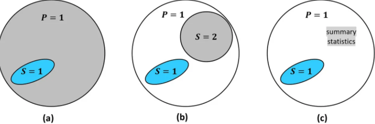
The sensitivity analyses require data on the distribution of pre-treatment covariates in the
target population. Such data may come from a full population (P= 1) dataset, a representative
(S= 2) sub-sample, or population summary statistics (seeFig 1).
Assumptions
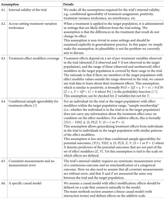
Several assumptions are required. The first assumption is that the trial has internal validity
(A1), which itself consists of several conditions listed inTable 1. We will not discuss interval
validity further, but this is a key assumption. On top of this, we need a set of assumptions
com-monly used in generalization [1–3]: across-setting treatment variance irrelevance (A2), trial
coverage of target population ranges of the effect modifiers (A3), conditional ignorability for treatment effects (A4), and consistent measurement and no measurement error (A5)—see
detailed explanations of and practical comments on these assumptions inTable 1.
Assumptions A1-A5 are sufficient for estimating TATE if all effect modifiers are observed in both the trial and target population, via either G-computation or weighting the trial sample
to the target population [1–3,11,12]. When some effect modifiers are not observed in the
tar-get population, however, such strategies fail. In this case, in order to use the proposed sensitiv-ity analyses to glean some information on TATE, we make the additional assumption (A6) of a
Fig 1. Several data source scenarios for generalization from the trial (S= 1) to the target population (P= 1). (a) the trial sample
and a full population dataset; (b) the trial sample and a dataset (S= 2) that is representative of the population; (c) the trial sample and some summary statistics about the population.
causal model. In this section we assume the linear causal model
E½YiðaÞ� ¼b0þbaaþbxXiþbzZiþbzaZiaþbvViþbvaVia; ðM1Þ
where potential outcomes are influenced by treatment conditionaand baseline covariates
X,Z,V, all observed in the trial.X,ZandVmay be multivariate; the use of univariate notation
is to simplify presentation.ZandVboth denote effect modifiers; the difference isZis observed
in the target population whileVis not.
(The letter M in the equation labelM1indicates that this is a causal model. We will also use
T in labels to indicate TATE formulas, and R to indicate regression models).
This model assumption should not be made lightly. With a binary outcome, for instance, this model would imply additive effects on the risk difference scale, which may be inappropriate.
Table 1. Key assumptions.
Assumption Details
A1. Internal validity of the trial We make all the assumptions required for the trial’s internal validity, e.g., conditional ignorability of treatment assignment, positivity, treatment variance irrelevance, no interference, etc.
A2. Across-setting treatment variation irrelevance
When a treatment is applied to the target population, it is administered in settings that are likely different from the trial setting. The
assumption is that the differences in the treatment that result do not change its effect.
This assumption is non-trivial in some settings and should be examined explicitly in generalization practice. In this paper, we simply make the assumption; its plausibility is not the problem we currently aim to discuss.
A3. Treatment effect modifiers coverage Treatment effects depend on a set of pre-treatment variables observed in the trial (denotedZif observed andVif not observed in the target population), and the range of these (observed and unobserved) effect modifiers in the target population is covered by their range in the trial. The rationale is that if there are members of the target population with effect modifier values outside the range observed in the trial, we cannot use trial data to learn about their treatment effects. This assumption, which is similar to positivity, is formally Pr(S= 1|Z=z,V=v)>0 if Pr (Z=z,V=v|P= 1)>0 where Pr[�] is the probability function [17]. This assumption can be checked forZvariables but not forV.
A4. Conditional sample ignorability for treatment effects [3]
For an individual (in the trial or the target population) with effect modifiers within the target population range, “sample membership” (i.e., whether the individual is in the trial or in the target population) does not carry any information about the treatment effect once we condition on the effect modifiers. For additive effects, this is formally [Y(1)−Y(0)]⫫{S,P}jZ,V, (S= 1 orP= 1).
This assumption allows generalizing treatment effects from individuals in the trial to individuals in the target population with similar patterns of the effect modifiers.
This assumption is less strict than conditional sample ignorability for potential outcomes, {Y(1),Y(0)}⫫{S,P}jX,Z,V, (S= 1 orP= 1) where
Xdenotes predictors of the potential outcomes that are not part of the set of effect modifiers {Z,V}. Yet this assumption is tied to the scale on which effects are defined.
A5. Consistent measurement and no measurement error
The trial’s internal validity requires no systematic measurement error of a continuous outcome and no misclassification of a categorical outcome. Here we also need to assume that all covariate measurements are without error, and thatXandZare measured the same way between the trial and the target population.
A6. A specific causal model We assume a causal model with effect modification; effects should be defined on a scale that connects naturally to the model.
The main methods section assumes a linear causal model (with interaction terms) and defines effects on the additive scale.
(See the next section for an extension of these methods to a broader class of models). Also, the selection of which pre-treatment variables to include in the model and which variables to con-sider effect modifiers requires serious investigation, and is discussed is great length in relevant
literature, e.g., [13–16]. With the current focus on sensitivity analysis, we presume that such a
model has been selected. If unsure whether a variable is an effect modifier (e.g., because its inter-action with treatment has a non-negligible coefficient but its p-value is large), our recommenda-tion is to treat it as one for the purpose of TATE estimarecommenda-tion, since trials usually lack power to investigate effect modification.
TATE formula
Based on the causal modelM1, individuali’s treatment effect has expectation E[Yi(1)−Yi(0)]
=βa+βzaZi+βvaVi, therefore
TATE¼baþbzaE½ZjP¼1� þbvaE½VjP¼1�; ðT1Þ
where E[Z|P= 1] and E[V|P= 1] are the means ofZandVin the target population. Under
Assumptions A1-A6,βa,βzaandβvaare the same for the trial sample and target population,
and can be estimated using trial data.
The problematic quantity in this formula is E[V|P= 1], because we do not observeVin
the target population. However, if we specify a plausible range for E[V|P= 1] (thesensitivity
parameter), we obtain a range of TATE estimates. We outline here two ways to do this, and
provide detailed implementation instructions inTable 2.
Method 1: Outcome-model-based sensitivity analysis
This method requires an estimate for E[Z|P= 1] (target population meanZ), but not a target
population dataset. It involves: (1) obtaining an estimate for E[Z|P= 1]; (2) specifying a
plausi-ble range for the sensitivity parameter E[V|P= 1]; (3) fitting to trial data the regression model
E½YjA;X;Z;V� ¼b0þbaAþbxXþbzaZAþbvVþbvaVA; ðR1Þ
(4) combining the estimated E[Z|P= 1] and specified E[V|P= 1] with model coefficients to
obtain TATE estimates (using formulaT1); and (5) plotting results against the sensitivity
parameter.
Method 2: Weighted-outcome-model-based sensitivity analysis
If a target population dataset is available, an alternative is to weight the trial sample to mimic
the target population distribution ofX,Z, before implementing the same steps as in method 1.
Simulations (see description and full results in theS1 Appendix) found that Method 2 has
an advantage over method 1 with respect to bias; it provides some protection against bias due to misspecification of the outcome model. Specifically, if the outcome model is misspecified
with respect toZ, method 1 is biased, but method 2 is unbiased because the weighting adjusts
for the difference between the trial and target population in effect variation due to the
differ-ence in distribution ofZ. Also, if the outcome model is misspecified with respect toVthen
both methods are biased, but ifVis positively correlated withZin the trial and influences
treatment effect in the same direction asZ, method 2 is less biased than method 1, because the
weighting adjustment forZhelps partially adjust forV. Method 2’s disadvantage is that it has
outcome model is correctly specified, with the method 1 confidence interval (CI) having nomi-nal coverage (about 95%) and the method 2 CI’s coverage being only slightly smaller (around 93-94%). When the outcome model is misspecified, due to bias reduction, method 2’s CI gen-erally has better variance than method 1’s.
Given these findings, we generally recommend method 2 (with the weighting), unless the two methods agree on TATE point estimates, in which case method 1’s unweighted results can be used.
Weighting procedures. Method 2 involves weighting the trial sample to mimic the target
population distribution ofX,Z. In most situations where a population dataset (eitherP= 1
orS= 2—seeFig 1) is available, we useweighting by the odds[3,18]. The exception is when
trial participants are part of AND can be identified within the population dataset, theninverse
probability weightingis used. If only population summary statistics are available, weighting is
generally not used. However, if information on the joint distribution ofX,Zin the target
pop-ulation is available, andX,Zare discrete with few combined categories, weighting may be
implemented. SeeTable 3for details on weights computation in these cases. For why they
apply, see theS2 Appendix.
Table 2. Implementation instructions.
Method 1: Outcome-model-based sensitivity analysis
Step 1 Obtain an estimate for E[Z|P= 1] (mean ofZin the target population), with confidence limits to reflect uncertainty (unless it is known with certainty, e.g., from a full population dataset).
Step 2 Specify a plausible range for E[V|P= 1] (aka thesensitivity parameter).
• This range should ideally be informed by knowledge about this variable from other data or from the literature regarding the target population or similar populations.
• When little information is available, a wide range can be used so that consumers of the research could be selective in interpreting the results based on information they may have on this parameter.
Step 3 Fit to the trial data the regression modelR1.
Step 4 For each of the lower and upper ends of the range specified for E[V|P= 1], obtain a corresponding estimate of TATE (including point estimate and confidence limits).
Suppose that for E[Z|P= 1], we have a point estimate of 2 and 95% confidence interval of (1.5, 2.5); and for E[V|P= 1], we specify a plausible range of 30 to 70. TATE corresponding to one end of this range, e.g., the lower end (E[V|P= 1] = 30), is estimated as follows:
• Point estimate: Take a linear combination of the coefficients from modelR1—based on the TATE formulaT1—using the point estimate 2 of E[Z|P= 1], that is, (βa+ 2βza+ 30βva). This can be done using thelincomstatement after fitting the model inStataor using theestimatestatement when specifying the model inSAS. The output for this linear combination includes a point estimate, standard error and confidence interval. Take the point estimate of this linear combination as the point estimate for TATE.
• Confidence limits: Use the confidence limits (1.5 and 2.5) of E[Z|P= 1] to take two additional linear combinations: (βa+ 1.5βza+ 30βva) and (βa+ 2.5βza+ 30βva). Consider the confidence limits of these linear combinations: take the more extreme of their two upper confidence limits, and the more extreme of their two lower confidence limits, as the confidence limits for TATE.
Step 5 Plot the range of TATE with confidence bounds (y-axis) against the range specified for the sensitivity parameter E[V|P= 1] (x-axis). Specifically,
• Plot the TATE estimates corresponding to the two ends of the range obtained in step 4, each with three points, one for the point estimate and two for the confidence limits; and
• Connect the two point estimates, the two lower confidence limits, and the two upper confidence limits, using three straight lines.
Method 2: Weighted-utcome-model-based sensitivity analysis
Step 0 Weight the trial sample so that it resembles the target population with respect toX,Z.
Steps 1-2
Same as in method 1
Step 3 Fit modelR1to the weighted trial sample.
Step 4-5 Same as in method 1
An additional note: The desired result of weighting is that the arms of the trial (i) each
mim-ics the target population in the distribution ofX,Z, and (ii) remain similar to each other in the
distribution ofX,Z,V. We recommend a two step procedure: first checking balance between
the trial arms and adjusting via within-trial reweighting if needed; and then weighting the (adjusted) trial sample to the target population. We do not recommend weighting each trial arm to the target population separately, because it may distort between-arms balance on vari-ables not observed in the target population.
What if an effect modifier is not even observed in the trial?
There are times when instead of an effect modifier observed in the trial but not in the target population, researchers are concerned about effect modifiers that were not measured in the trial. This may be a specific variable, e.g., addiction severity was not measured in a substance abuse treatment trial, but it is suspected to modify treatment effect and it may very well be dis-tributed differently between the trial and the target population. Or it may be generic, when researchers are concerned that there is effect modification by unknown factors.
The question is whether the above-described sensitivity analyses can be extended to cover
an effect modifierU(be it a specific or generic variable) that is unobserved in the trial.
Unfor-tunately, the answer is no. It is clear from the causal model
E½YiðaÞ� ¼b0þbaaþbxXiþbzZiþbzaZiaþbuUiþbuaUia
that if we use the approach without weighting, we would need an estimate ofβza, which is
Table 3. Weighting procedures for different target population data scenarios. Target population data Weighting procedures
AP= 1 dataset is available. Trial participants cannot be identified in thisP= 1 dataset.
Weighting-by-the-odds, i.e., weight the trial participants using weights computed as follows
1. stacking the trial and target population datasets into one dataset, and creating a new variableS0codedS0= 1 for
observations from the trial dataset, andS0= 0 for observations
from the target population dataset
2. fitting a model usingXandZto predictS0; and for each trial
participant, obtaining the predicted probability ofS0= 1 from
that model (aka the trialparticipation score),psi= Pr(S0= 1|
Xi,Zi)
3. for every trial participant, computing the weights asWi= (1−
psi)/psi, the odds of being in the target population dataset. AS= 2 dataset is available. Trial participants are
either not part of theS= 2 sample, or if they are, they cannot be identified in thisS= 2 dataset.
AP= 1 dataset is available. Trial participants are identified in thisP= 1 dataset.
Inverse-probability-weighting, i.e., weight the trial participants using weights computed as follows
1. using the target poplation dataset, creating a new variableS0
codedS0= 1 for observations that belong to the trial
participants, andS0= 0 for the remaining observations
2. fitting a model usingXandZto predictS0; and for each trial
participant, obtaining the predicted probability ofS0= 1 from
that model (aka the trialparticipation score),psi= Pr(S0= 1|
Xi,Zi)
3. for every trial participant, computing the weights asWi= 1/
psi, the inverse of the probability of participating in the trial. AS= 2 dataset is available. Trial participants are
part of theS= 2 sample, and are identified in this
S= 2 dataset.
Information on the joint distribution of {X,Z} in the target population is available.
X,Zare categorical with a small number of combined categories.
Ratio-of-probability-weighting, specifically, weight the trial participants using weights computed by the formula
Wi¼
PrðX¼Xi;Z¼ZijP¼1Þ
PrðX¼Xi;Z¼ZijS¼1Þ
, where the numerator and
denominator are the prevalences of the {Xi,Zi} pattern in the target population and in the trial sample, respectively.
unidentified from the trial becauseUis not observed. If we use the weighting approach and
manage to equate the mean ofZbetween the trial sample and the target population, then we
could do withoutβzabut instead would have to deal with the mean ofUin the weighted trial
sample, an obscure quantity that is not suitable to serve as a sensitivity parameter. (For
techni-cal details, see theS3 Appendix).
Note that this is a correction of theUcase results reported in [6]; the appendix explains the
error in those previous results.
Method extensions
Turning our attention back to effect modifiers that are observed in the trial but not in the
tar-get population (V), note that the last section (and [6]) addressed a simple setting. We now
offer two extensions of the sensitivity analyses to more complex situations.
Extension 1: When both pre- and post-treatment outcomes are available
and are modeled using random intercepts models
When both pre- and post-treatment measures of the outcome are available, there are several options for modeling such data. One option is to treat the pre-treatment outcome measure as a baseline covariate. Another option, which we consider here, is to model the combination of both pre- and post-treatment outcomes using random intercepts models.
The simplest random intercepts model in this case is the model without covariates
E½YijjAi;Fij� ¼c0iþg0þgaAiþgfFijþgfaFijAi;
whereiindexes person,jindexes observation (each person has two observations),Aindicates
treatment arm,Findicates whether the observation is pre-treatment (Fi1= 0) or
post-treat-ment (Fi2= 1), and the coefficientγfaofFArepresents treatment effect. Given randomization
of treatment in the trial, when this model is fit to the trial data,γfaestimates SATE. Note that
the coefficient ofFAin models with baseline covariates (X,Z,V) that may interact withAorF
but not withFAalso estimates SATE; such models adjust for covariates when estimating the
average treatment effect.
For the sensitivity analyses, we assume a model with effect modification analogous toM1.
The full details, which are somewhat more complicated than are informative, are relegated to theS4 Appendix. The key point is that this model includes not only theFAterm (βfaFijAi),
but also interaction terms of effect modifiers withFA(βzfaZiFijAiandβvfaViFijAi). The
TATE formula in this case is
TATE¼bfaþbzfaE½ZjP¼1� þbvfaE½VjP¼1�: ðT2Þ
This formula is used with both method 1 and method 2—when the effect modification regression model is fit to the unweighted and weighted trial data, respectively.
While it is usually natural to clarify effect definitions before discussing models used to esti-mate such effects, in this section we have done the opposite, starting with models first. This choice is intentional because in the current case it is easier to point out the effect definition
after explaining the model. AsFAis an interaction of treatment arm and time (post- vs.
on the potential post-treatment outcome. That is, the TATE and SATE in this case are exactly the same average effects defined in the previous section.
Extension 2: Multiplicative effects on potential outcome rate/probability/
odds, based on a log/logit link model
In the previous section, we commented that the linear model assumption is not always appro-priate. We now extend the methods to cases where log/logit link outcome models are used (e.g., log mean model for a count outcome, log probability or logit model for a binary out-come). Here the individual treatment effect is defined on the multiplicative scale that matches the model (e.g., rate ratio, risk ratio, or odds ratio), and an ATE is defined as the geometric mean of the individual effects. Or equivalently, one could define the individual effect as the corresponding log rate ratio, log risk ratio or log odds ratio, and have the usual definition of ATE as the arithmetic mean of individual effects.
We describe the extension formally here using a binary outcome with logit model (leaving
details for the other cases in theS5 Appendix). In this case we assume the logistic causal model
log Pr½YiðaÞ ¼1�
Pr½YiðaÞ ¼0�
� �
¼b0þbaaþbxXiþbzZiþbzaZiaþbvViþbvaVia; ðM3Þ
the coefficients of which can be estimated by fitting the logistic regression model
log Pr½Y ¼1jA;X;Z;V� Pr½Y ¼0jA;X;Z;V�
� �
¼b0þbaAþbxXþbzZþbzaZAþbvVþbvaVA ðR3Þ
to the original or the weighted trial sample (corresponding to method 1 or 2). Define the indi-vidual treatment effect as the odds ratio (OR) of the indiindi-vidual’s potential outcomes,
TEORi ¼
Pr½Yið1Þ ¼1�=Pr½Yið1Þ ¼0�
Pr½Yið0Þ ¼1�=Pr½Yið0Þ ¼0� ;
or the corresponding log OR
TElog OR
i ¼logðTE
OR
i Þ:
ModelM3implies,
TElog OR
i ¼baþbzaZiþbvaVi;
TEOR
i ¼ expðbaþbzaZiþbvaViÞ:
On the log OR scale, we have the familiar formula
TATElog OR ¼b
aþbzaE½ZjP¼1� þbvaE½VjP¼1� ðT3aÞ
for TATE defined as the average of the individual effects in the target population. Note that ‘average’ in this definition means arithmetic mean. For effects defined on the OR scale, how-ever, the arithmetic mean does not have a nice formula. Yet we can use another type of average that is natural to quantities on a multiplicative scale and thus is both meaningful and mathe-matically convenient in this case, the geometric mean. Defining TATE on the OR scale as the geometric mean of the individual ORs in the target population, we obtain
TATEOR¼ expfb
These two TATE formulas serve as the basis for essentially the same sensitivity analyses, as
TATEOR= exp(TATElog_OR).
As an aside, an ATE defined as geometric mean of individual OR effects (termedaverage
causal OR) is closely related to the conditional OR routinely estimated by logistic regression with main effects only. Indeed the latter is an approximate estimate of the former (see more
about this in theS5 Appendix).
Illustration
The analyses presented here are merely illustrative. Results should not be taken as clinically informative. In addition to the concise presentation here, the detailed analyses can be found in
S6 Appendix, with most of the code (R-code) included in the same appendix, and some Stata
code inS7 Appendix. The data are provided inS8andS9Appendices.
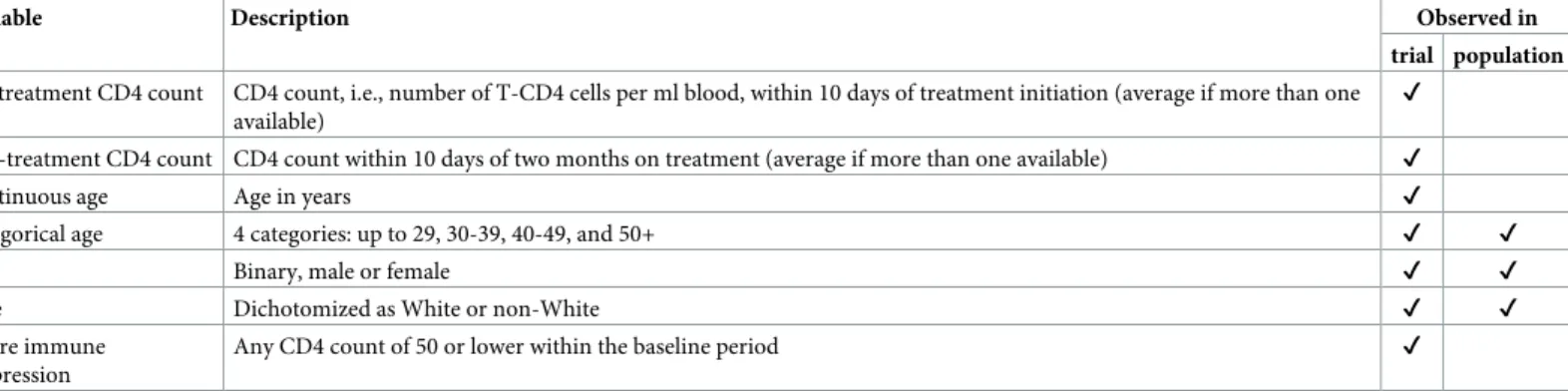
The trial data include baseline and post-treatment CD4 counts and several baseline char-acteristics—age in years, sex, race, and severe immune suppression (SIS). The target
popula-tion data include age groups, sex, and race. SeeTable 4for a description of these variables.
As noted above, when data include pre- and post-treatment measures of the outcome, there are more than one analysis options. Here we use random intercepts models on the
combina-tion of both measures. (For an applicacombina-tion modeling post-treatment outcome only, see [6]).
The definition of TATE is the average effect of treatment on potential CD4 count gain, and equivalently, the average effect of treatment on potential CD4 count post-treatment, in the target population.
We start by analyzing the trial data. The first question is whether to model CD4 count (and thereby consider its change) on the additive or multiplicative scale. CD4 count is a non-nega-tive variable, so the addinon-nega-tive scale may predict out of range, but it is also generally bounded above, which is more restrictive on multiplicative than on additive effects. We follow the HIV literature convention of using the additive scale for CD4 count, noting that our models may be suboptimal in this respect.
The two treatment arms in the trial are similar but the new treatment arm has more female
patients and the old treatment arm has a higher SIS proportion (seeTable 5). For the moment,
assume we have good enough balance; we will come back to this.
SATE (i.e., the average difference, between the two treatments in the trial, in CD4 count change, or equivalently, in post-treatment CD4 counts) is estimated to be 36.6, 95% CI = (28.0,45.2) cells/ml by a simple model with no covariates, and 35.8, 95% CI = (27.3,44.4) by a
model that adjusts for baseline covariates.Table 6shows substantial differences in covariate
Table 4. Illustration. Data availability.
Variable Description Observed in
trial population
Pre-treatment CD4 count CD4 count, i.e., number of T-CD4 cells per ml blood, within 10 days of treatment initiation (average if more than one available)
✔
Post-treatment CD4 count CD4 count within 10 days of two months on treatment (average if more than one available) ✔
Continuous age Age in years ✔
Categorical age 4 categories: up to 29, 30-39, 40-49, and 50+ ✔ ✔
Sex Binary, male or female ✔ ✔
Race Dichotomized as White or non-White ✔ ✔
Severe immune suppression
Any CD4 count of 50 or lower within the baseline period ✔
distribution between the trial sample and target population, suggesting these SATE estimates should not be used as estimates of TATE.
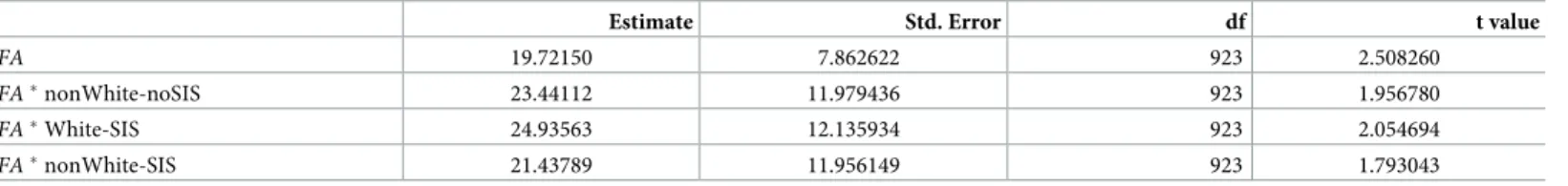
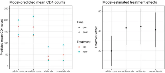
Through a simple analysis examining interactions ofFAwith baseline covariates (e.g.,
FA�sex), covariate pairs (e.g.,FA�sex�age), and cross-classifications of categorical covariates
(e.g.,FA�‘nonwhite-female’), we identify that the cross-classification of race and SIS status is
an effect modifier (seeTable 7). This variation in treatment effects is visualized inFig 2.
As treatment effects vary across race-by-SIS-status categories, to obtain TATE estimates, we need the proportions of the target population that are in these categories. Race is observed in the target population, with 63.9% being nonwhite. SIS status (in the white and nonwhite groups), however, is not observed. If this were a substantive study, we would comb the litera-ture to seek a plausible range for the proportions with SIS among White and among nonWhite people in the target population. As this is only illustrative, we specify a wide range (0.2, 0.6) for this proportion (which covers the proportion 0.456 in the trial), and assume that this propor-tion is the same between White and nonWhite people in the target populapropor-tion. With this
assumption, this single proportion with SIS in the target population is now oursensitivity
parameter.
Table 6. Illustration. Covariate distribution in the trial sample and target population. Trial sample
(n = 933)
Target population (n = 54,220)
Age (mean) 39.5 not available
Age (range) 16 to 75 13 to 80
Age groups (proportions)
29 and younger 0.107 0.341
30 to 39 0.421 0.309
40 to 49 0.348 0.247
50 and older 0.123 0.103
Sex (proportion female) 0.159 0.266
Race (proportion nonWhite) 0.471 0.639
SIS (proportion) 0.456 not available
https://doi.org/10.1371/journal.pone.0208795.t006
Table 5. Illustration. Covariate balance within the trial sample.
New treatment (n = 478)
Old treatment (n = 455)
Age (mean) 39.4 39.5
Sex (proportion female) 0.174 0.143
Race (proportion nonWhite) 0.473 0.468
SIS (proportion) 0.437 0.475
https://doi.org/10.1371/journal.pone.0208795.t005
Table 7. Illustration. Excerpt from effect modification modelafit to trial data.
Estimate Std. Error df t value
FA 19.72150 7.862622 923 2.508260
FA�nonWhite-noSIS 23.44112 11.979436 923 1.956780
FA�White-SIS 24.93563 12.135934 923 2.054694
FA�nonWhite-SIS 21.43789 11.956149 923 1.793043
a
The referent category is White-noSIS. The other covariates included are age and sex.
A comment is warranted on assumption A3, that the range of the treatment effect modifiers in the target population is covered by the trial. In the current example, it is apparent that we do not have a problem with this assumption, because effect modification involves the four race-by-SIS-status categories, all of which are present in the trial sample. What might go unnoticed is that the age range in the trial sample (16 to 75) is smaller than that in the target population (13 to 80), and while we did not detect any treatment effect modification by age in the trial sample, we do not know if treatment effects for those younger than 16 or older than 75 (who are not represented in the trial sample) are the same as or different from treatment effects for those in the trial sample age range; this would be an area to consult clinical experts for their judgment. In the absence of such expert knowledge, were actual age values (rather than just age group) observed in the target population, one option would be to generalize treatment effects only to those aged 16 to 75 in the target population. This target population trimming is not an option in the current case as age values are not observed. In order to move forward, we assume that there is no effect modification by age.
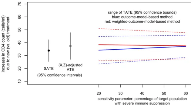
We now apply theoutcome-model-based sensitivity analysis(method 1) with the specified
(0.2, 0.6) range for the sensitivity parameter (proportion with SIS in the target population). This obtains a range of TATE estimates from 36.2, 95% CI = (25.9,46.6) (corresponding to the lower end of the sensitivity parameter range) to 39.3, 95% CI = (30.0,48.6) (corresponding to the upper end of the sensitivity parameter range).
To apply theweighted-outcome-model-based sensitivity analysis(method 2), we need to
weight the trial data to mimic the target population with respect to covariates observed in both (age group, sex, race). Heeding the recommendation of the two-step procedure, we first adjust the between-arms balance in the trial sample by inverse treatment propensity score weighting. Note that this results in a balance-adjusted SATE estimate of 33.9, 95% CI = (25.4, 42.3), which is very similar to (but slightly smaller than) the original SATE estimates. The effect modifica-tion model fit to the balance-adjusted trial data is very similar to that fit to the raw trial data. If we use that model and apply method 1, we obtain TATE estimates ranging from 34.2, 95% CI = (23.5, 44.8) to 37.1, 95% CI = (28.5, 45.7); these are slightly lower than those based on the model fit to the raw data. To use method 2, after adjusting within-trial balance, we weight the adjusted trial sample to the target population, using the weighting-by-the-odds procedure
described inTable 3. This results in covariate balance shown inTable 8. The ATE in this
Fig 2. Illustration. Visualization of effect modification model.
weighted trial sample (which we will refer to as the (X,Z)- adjusted ATE) is 37.4, 95% CI = (27.0, 47.8), which is slightly higher than our SATE estimates. This is consistent with the fact that the weighted trial sample has higher nonWhite and SIS proportions than the original trial sample.
We now fit the same effect modification model to the weighted trial sample (see model fit inTable 9). Interestingly, the coefficients have changed substantially from the model fit to raw
data (Table 7). This is not surprising as it could be a result of model misspecification (which
we suspected), and it underscores our recommendation to use the weighted method so that the model that is the basis for estimating (sensitivity analysis of) TATE is the model fit to data that is close to the target population with respect to observed variables.
Generally we should not read much into the (lack of) statistical significance of interaction terms in the weighted model because weighting increases variance. However, the underwhelm-ing coefficients in the fitted model above suggest that in the weighted dataset, there is not
much differentiation of the group specific effects, and one could argue for using the (X,Z
)-adjusted ATE as an estimate of TATE.
Or we could choose to proceed with a full implementation of method 2. Based on this effect modification model, we obtain TATE estimates ranging from 38.4, 95% CI = (26.0,50.9) (cor-responding to the lower end, 0.20, of the range of the sensitivity parameter) to 37.5, 95% CI = (27.4,47.7) (corresponding to the upper end, 0.60, of the range of the sensitivity parameter).
Results from both methods are plotted inFig 3. In this particular case, as there is not a clear
slope of TATE estimates on the sensitivity parameter, we could combine these results to con-clude that when between 20 and 60% of the target population have SIS, we could expect the tar-get population average effect of the new treatment (relative to the old treatment) to be a gain in CD4 count of about 36 to 39 cells per ml (point estimate) with lower and upper confidence bounds of 26 and 51.
Table 8. Illustration. Covariate balance between two trial arms and target population after weighting. Trial: new
(n = 478)
Trial: old (n = 455)
Target population (n = 54,220)
Age (mean) 35.8 36.1 not available
Age (range) 16 to 75 16 to 75 13 to 80
Age groups (proportions)
29 and younger 0.349 0.333 0.341
30 to 39 0.304 0.313 0.309
40 to 49 0.247 0.246 0.247
50 and older 0.100 0.107 0.103
Sex (proportion female) 0.272 0.260 0.266
Race (proportion nonWhite) 0.642 0.636 0.639
SIS (proportion) 0.515 0.522 not available
https://doi.org/10.1371/journal.pone.0208795.t008
Table 9. Illustration. Excerpt from effect modification model fit to trial data that have been weighted to the target
population.
Estimate Std. Error z value
FA 32.903852 11.93896 2.76
FA�nonWhite-noSIS 9.335134 15.74757 0.59
FA�White-SIS 4.593148 14.53369 0.32
FA�nonWhite-SIS 3.294465 15.46597 0.21
Discussion
Policy-makers may want to use trial results to inform decisions for specific target populations. There are now methods to calibrate trial results to target populations, increasing potential for
evidence-based decision-making [19]. However, these methods generally rely on a strong
assumption that all effect modifiers differentially distributed between sample and population are observed and can be adjusted for. In this paper, we describe sensitivity analyses when this is not the case. Sensitivity analyses such as these allow researchers and decision-makers to have more appropriate confidence about population effects.
The methods proposed in this paper address situations where the effect definition matches the model assumed—additive effect with linear model, ratio effect with logit/log link model. While this kind of pairing is natural and commonplace, it is somewhat restrictive; there are sit-uations where the effect definition of policy interest may not be on the same effect scale that best matches the model scientifically deemed appropriate. Our ongoing work aims to provide sensitivity analyses to situations where the model assumed is nonlinear but the effect scale of interest is additive.
That these sensitivity analyses rely on the assumption of a specific causal model deserves discussion, as the assumed model may or may not be close to the truth. Method 2, which com-bines this model with weighting, provides some protection against model misspecification, and thus has a flavor of double robustness. It is not truly doubly robust, however, because the weighting does not adjust for difference in the distribution of the partially unobserved effect
modifierV. An area for further development is the search for sensitivity analysis procedures
that are more flexible regarding model assumptions.
A challenge in generalization which we commented on is that the effect modifier range cov-erage assumption (A3) is perhaps commonly not met, because trial samples tend to be less
diverse than target populations [20]. Strategies for this situation include combining evidence
from multiple trials, combining experimental and non-experimental evidence using
cross-Fig 3. Illustration. Results from both methods.
design synthesis [21], or redefining the population to the area with overlap [22]. These com-plex approaches will require adapting sensitivity analyses.
Finally, it is important to note that these sensitivity analyses are not a panacea. It is best to limit the need for them in the first place. This can be done through careful consideration of tar-get populations when designing trials, and efforts to enroll more representative trial samples. If that is not possible, trialists should carefully consider potential effect modifiers and investi-gate treatment effect heterogeneity. Also, to be able to adjust for effect modifiers when general-izing treatment effects, effect modifiers need to be measured consistently in trials and target
population datasets [5,23]. We encourage trialists to collect covariates in the same way as is
done in common population datasets in their fields. When design strategies fall short, the methods discussed here provide a sense for the robustness (or lack thereof) of results when generalizing to target populations.
Supporting information
S1 Appendix. Simulations.
(PDF)
S2 Appendix. An explanation of why the different weighting procedures apply in the dif-ferent data scenarios.
(PDF)
S3 Appendix. Additional details on the case of effect modifiers not observed in the trial.
(PDF)
S4 Appendix. Additional details on extension 1 for random intercepts models.
(PDF)
S5 Appendix. Additional details on extension 2 for multiplicative effects and log/logit link models.
(PDF)
S6 Appendix. Illustration—Main appendix with explanations and most of the code in R (read this before S7-9).
(HTML)
S7 Appendix. Illustration—Stata code for fitting random effects models with probability weights.
(DO)
S8 Appendix. Illustration—Trial data.
(CSV)
S9 Appendix. Illustration—Target population data.
(CSV)
Acknowledgments
Author Contributions
Conceptualization: Trang Quynh Nguyen, Stephen R. Cole, Elizabeth A. Stuart.
Data curation: Trang Quynh Nguyen.
Formal analysis: Trang Quynh Nguyen.
Funding acquisition: Elizabeth A. Stuart.
Investigation: Trang Quynh Nguyen.
Methodology: Trang Quynh Nguyen, Elizabeth A. Stuart.
Supervision: Elizabeth A. Stuart.
Visualization: Trang Quynh Nguyen.
Writing – original draft: Trang Quynh Nguyen.
Writing – review & editing: Trang Quynh Nguyen, Benjamin Ackerman, Ian Schmid,
Ste-phen R. Cole, Elizabeth A. Stuart.
References
1. Cole SR, Stuart EA. Generalizing evidence from randomized clinical trials to target populations: The ACTG 320 trial. American Journal of Epidemiology. 2010; 172(1):107–115.https://doi.org/10.1093/aje/
kwq084PMID:20547574
2. Tipton E. Improving generalizations from experiments using propensity score subclassification: Assumptions, properties, and contexts. Journal of Educational and Behavioral Statistics. 2013; 38 (3):239–266.https://doi.org/10.3102/1076998612441947
3. Kern HL, Stuart EA, Hill JL, Green DP. Assessing methods for generalizing experimental impact esti-mates to target samples. Journal of Research on Educational Effectiveness. 2016; 9(1):103–127.
https://doi.org/10.1080/19345747.2015.1060282PMID:27668031
4. Stuart EA, Bradshaw CP, Leaf PJ. Assessing the generalizability of randomized trial results to target populations. Prevention Science. 2015; 16(3):475–485.https://doi.org/10.1007/s11121-014-0513-z PMID:25307417
5. Stuart EA, Rhodes A. Generalizing treatment effect estimates from sample to population: A case study in the difficulties of finding sufficient data. Evaluation Review. 2016.https://doi.org/10.1177/
0193841X16660663PMID:27491758
6. Nguyen TQ, Ebnesajjad C, Cole SR, Stuart EA. Sensitivity analysis for an unobserved moderator in RCT-to-target-population generalization of treatment effects. Annals of Applied Statistics. 2017; 11 (1):225–247.https://doi.org/10.1214/16-AOAS1001
7. Hammer SM, Squires KE, Hughes MD, Grimes JM, Demeter LM, Currier JS, et al. A controlled trial of two nucleoside analogues plus indinavir in persons with human immunodeficiency virus infection and CD4 cell counts of 200 per cubic millimeter or less. New England Journal of Medicine. 1997; 337 (11):725–733.https://doi.org/10.1056/NEJM199709113371101PMID:9287227
8. Hall HI, Song R, Rhodes P, Prejean J, An Q, Lee LM, et al. Estimation of HIV incidence in the United States. JAMA: The journal of the American Medical Association. 2008; 300(5):520–9.https://doi.org/10.
1001/jama.300.5.520PMID:18677024
9. Pearl J, Bareinboim E. External validity and transportability: A formal approach. JSM Proceedings. 2011; p. 157–171.
10. Rubin DB. Estimating causal effects of treatments in randomized and nonrandomized studies. Journal of Educational Psychology. 1974; 66(5):688–701.https://doi.org/10.1037/h0037350
11. Pressler TR, Kaizar EE. The use of propensity scores and observational data to estimate randomized controlled trial generalizability bias. Statistics in Medicine. 2013; 32(20):3552–3568.https://doi.org/10.
1002/sim.5802PMID:23553373
13. Kent DM, Rothwell PM, Ioannidis JPA, Altman DG, Hayward RA. Assessing and reporting heterogene-ity in treatment effects in clinical trials: A proposal. Trials. 2010; 11:85.
https://doi.org/10.1186/1745-6215-11-85PMID:20704705
14. Wang R, Ware JH. Detecting moderator effects using subgroup analyses. Prevention Science. 2013; 14:111–120.https://doi.org/10.1007/s11121-011-0221-xPMID:21562742
15. Weiss MJ, Bloom HS, Brock T. A conceptual framework for studying the sources of variation in program effects. Journal of Policy Analysis and Management. 2014; 33(3):778–808.https://doi.org/10.1002/ pam.21760
16. Varadhan R, Segal JB, Boyd CM, Wu AW, Weiss CO. A framework for the analysis of heterogeneity of treatment effect in patient-centered outcomes research. Journal of Clinical Epidemiology. 2013; 66 (8):818–825.https://doi.org/10.1016/j.jclinepi.2013.02.009PMID:23651763
17. Lesko CR, Buchanan AL, Westreich D, Edwards JK, Hudgens MG, Cole SR. Generalizing study results: A potential outcomes perspective. Epidemiology. 2017;.https://doi.org/10.1097/EDE.
0000000000000664
18. Westreich D, Edwards JK, Lesko CR, Stuart EA, Cole SR. Transportability of trial results using inverse odds of sampling weights. American Journal of Epidemiology. 2017; 186(8):1010–1014.https://doi.org/
10.1093/aje/kwx164PMID:28535275
19. Westreich D, Edwards JK, Rogawski ET, Hudgens MG, Stuart EA, Cole SR. Causal impact: Epidemio-logical approaches for a public health of consequence. American Journal of Public Health. 2016; 106 (6):1011–1012.https://doi.org/10.2105/AJPH.2016.303226PMID:27153017
20. Humphreys K, Weingardt KR, Harris AHS. Influence of subject eligibility criteria on compliance with National Institutes of Health guidelines for inclusion of women, minorities, and children in treatment research. Alcoholism: Clinical and Experimental Research. 2007; 31(6):988–995.https://doi.org/10. 1111/j.1530-0277.2007.00391.x
21. Kaizar EE. Estimating treatment effect via simple cross design synthesis. Statistics in Medicine. 2011; 30(25):2986–3009.https://doi.org/10.1002/sim.4339PMID:21898521
22. Tipton E, Fellers L, Caverly S, Vaden-Kiernan M, Borman G, Sullivan K, et al. Site selection in experi-ments: An assessment of site recruitment and generalizability in two scale-up studies. Journal of Research on Educational Effectiveness. 2016; 9(sup1):209–228.https://doi.org/10.1080/19345747. 2015.1105895