Analysis of Manipulators Using SDRE: A Closed Loop Nonlinear Optimal Control Approach

Analysis of Manipulators Using SDRE: A Closed

Loop Nonlinear Optimal Control Approach

M.H. Korayem

_{, M. Irani}

_{and S. Rafee Nekoo}

Abstract. In this paper, the State Dependent Riccati Equation (SDRE) method is implemented on robotic systems such as a mobile two-links planar robot and a xed 6R manipulator with complicated dynamic equations. Dynamic modelings of both cases are presented using the Lagrange method. Afterwards, the Dynamic Load Carrying Capacity (DLCC), which is an important characteristic of robots, is calculated for these two systems. DLCC is calculated for the predened end-eector path, where motor torque limits and tracking error constraints are imposed for this calculation. For a mobile two-links planar robot, the stability constraint is discussed by applying a zero moment point approach. A nonlinear feedback control law is designed for the fully nonlinear dynamics of two cases using a nonlinear closed-loop optimal control method. For solving the SDRE equation that appears in the optimal control solution, a power series approximation method is applied. DLCC is obtained, subject to accuracy and torque constraints, by applying this feedback control law for the square and linear path of the end-eector for mobile two-link and a 6R manipulator, respectively. Finally, simulations are done for both cases and the DLCC of manipulators is determined. Also, actual end-eector positions, required control eorts and the angular position and velocity of joints are presented for full load conditions, and results are discussed

Keywords: Mobile manipulator; 6R robot; Nonlinear optimal control; DLCC; SDRE.

INTRODUCTION

In the last few years, developments in the industrial production of complicated parts and the importance of rapid productions, lead to automatic manufactur-ing. Manipulators and robot arms helped to achieve this purpose. Furthermore, some activities, like the transportation of heavy pieces and work in dangerous environments and large spaces, led to the use of mobile robots and manipulators.

Whereas mobile manipulators have a higher de-gree of freedom path planning, the trajectory control and determining of the important parameters of a robot are complicated. One of these important parameters is the Dynamic Load Carrying Capacity (DLCC), the load that a robot can repeatedly lift and carry on a de-sired trajectory. Korayem and Pilechian [1] calculated the DLCC of exible joint robots using a sliding mode

1. Robotic Research Laboratory, College of Mechanical Engi-neering, Iran University of Science and Technology, Tehran, P.O. Box 18846, Iran.

*. Corresponding author. E-mail: [email protected] Received 31 January 2010; received in revised form 11 June 2010; accepted 6 September 2010

control for the trajectory tracking problem. Korayem et al. [2] presented the DLCC of exible joint robots with a feedback linearization method and compared it with an open loop method. Also, Korayem and Irani [3] found the DLCC of mobile manipulators using a nonlin-ear optimal feedback controller. The solution method is a successful approximation for solving optimal control problems.

In [4], the Iterative Linear Programming (ILP) method is used to solve the optimization problem of nding the DLCC of cable driven robots. The results of the ILP method are then compared with the optimal control method.

In [5], the DLCC of a exible link manipulator mounted on a vehicle is determined via a feedback linearization control approach. Korayem et al. [6] calculated the maximum allowable load for a exible link manipulator with a mobile base, applying the nite element approach. This approach is applied to linear and circular trajectories.

Korayem et al. [7] established the maximum load carrying capacity of a mobile robot in an environment with obstacles using an open loop optimal control approach and considered stability constraint. The

stability constraint was measured by computing the zero moment point.

In this paper, the optimal control method is used to design a nonlinear closed loop control law for both xed and mobile manipulators. A proper approach in the nonlinear optimal control method is the SDRE method, based on solving the nonlinear state-dependent Riccati equation. Being simple and systematic are two advantages of this solution method. Also, this method is applicable to fully nonlinear dynamic models. Pearson [8] proposed the SDRE method, which was, then, developed by Wernli and Cook [9]. Then, SDRE was used as nonlinear opti-mal regulator. Cloutier [10] presented this method with state constraint and compared it with an LQR approach. In [11], the SDRE method is used to synthesize a path controller, and then the simulation results were checked by experimental results using real hardware. Innocenti et al. [12] presented the SDRE method to control a two-link under-actuated robot and described that, with the same designing parameters, the SDRE control can perform better than the LQR control.

Xin et al. [13] used the SDRE method to control a robot. An extra controller based on a neural network is used in the presence of parameter uncertainties to provide robustness characteristics. Shawky et al. [14] represented this method for a exible link manipulator. For this purpose, the Lagrange and assume mode methods are used for nding the dynamic model. Singh et al. [15] expressed the control of an inverted pendulum on a cart using the SDRE method; dierent values for weighing matrixes are used and results are compared. In [16] Cimen presented an overview on SDRE with details on stability, optimality and etc. Beikzadeh and Taghirad [17] used this for controlling a permanent magnet synchronous motor.

The exact solution of an SDRE equation is possible for a simple system, but for complicated systems, solving SDRE is dicult and is usually done using numerical methods. In this paper, a power series approximation is applied to solve this problem. The second section presents the method of solving a nonlinear optimal control problem using the SDRE approach. Then, in the next section, the power series approximation method is applied for solving the complex Riccati equation that appeared in the SDRE method. The denitions of a dynamic load carrying capacity and zero moment point are exposed in the next section. Afterwards, the dynamic modeling of a planar, 2-link mobile manipulator and a six degree of freedom manipulator are considered. The last section deals with the implementation of the SDRE method for a mobile manipulator and a 6R robot, and then results for a predened trajectory are demon-strated.

STATE-DEPENDENT RICCATI EQUATION Consider a nonlinear equation of a system as below:

_x = f(x(t)) + B(x(t))u(t); x(0) = x0; (1)

where x and u are state and input vectors, respec-tively, x 2 Rn _{and u 2 R}m_{, f : R}n _{! R}n_{, and}

B : Rn _{! R}nm _{are nonlinear functions and x0 is}

initial condition. The performance index that must be minimized is of the form:

J = Z ₁

0 (x

T_{(t)Q(x)x(t) + u}T_{(t)R(x)u(t))dt; (2)}

where Q 2 Rnn _{is Symmetric Positive Semi-Denite}

(SPSD), and R 2 Rmm_{is Symmetric Positive Denite}

(SPD). Rewriting the nonlinear equation in the State-Dependent Coecient (SDC) form becomes [18]:

_x = A(x)x(t) + B(x)u(t): (3)

Then the optimal solution of Equation 3, which min-imizes the performance index, is obtained from the following equation [18]:

X(x)A(x) + AT_(x)X(x)

X(x)B(x)R 1_(x)BT_{(x)X(x) + Q = 0: (4)}

This equation is named the state-dependent Riccati equation, where X is symmetric positive denite, which is the solution of the SDRE equation. Also, the state feedback control law is obtained in the following form:

u(x) = R 1_(x)BT_{(x)X(x)x: (5)}

POWER SERIES APPROXIMATION METHOD FOR SOLVING SDRE

For nding the numerical solution of SDRE, consider a system with Equation 3 where B is a constant matrix. By rewriting A in the following form [19];

A(x) = A0+ "A(x); (6)

and representing X as a Taylor series: X(x; ") =

1

X

n=0

"n_L n(x)

= X(x)

"=0

" +@2_@"X(x)₂

"=0

"2

and substituting A(x), X(x; ") into the SDRE equa-tion, the result will be in the following form:

1

X

n=0

"n_L n(x)

!

:(A0+ "A(x))

+ (A0+ "A(x))T 1

X

n=0

"n_L n(x)

!

1

X

n=0

"n_L n(x)

!

BR 1_BT X1 n=0

"n_L n(x)

!

+ Q = 0: (8)

By expanding this equation and collecting a similar power of ", three iterative equations are generated:

L0A0+ AT0L0 L0BR 1BTL0+ Q = 0; (9)

L0A(x) + A(x)TL0+ L1(A0 BR 1BTL0)

+ (AT

0 L0BR 1BT)L1= 0; (10)

Ln 1A(x) + A(x)TLn 1

+ Ln(A0 BR 1BTL0)

+ (AT

0 L0BR 1BT)Ln n 1

X

m=1

LmBR 1BTLn m = 0; (11)

where n = 2; 3; 4; .

The rst equation is an Algebraic Riccati Equa-tion (ARE), the second and third are state-dependent Lyapunov equations. These equations are simplied by substitution:

A(x) = g(x)A :

L0A0+ AT0L0 L0BR 1BTL0+ Q = 0; (12)

L0A + ATL0+ L1(A0 BR 1BTL0)

+ (AT

0 L0BR 1BT)L1= 0; (13)

Ln 1A + ATLn 1+ Ln(A0 BR 1BTL0)

+ (AT

0 L0BR 1BT)Ln n 1

X

m=1

LmBR 1BTLn m= 0: (14)

Similarly, the state-feedback control law is obtained: u = R 1_BT X1

n=0

gn_(x)L

nx: (15)

For most complicated systems, A(x) could not be rewritten as A(x) = g(x)A. For these systems, A(x) is changed to:

A(x) = A0+ j

X

i=1

fi(x)Ai; (16)

where j is the number of nonlinear terms, and fi(x) and

Aiare constant matrixes. Also, L1can be written as:

L1= j

X

i=1

fi(x)Lj1: (17)

Using two prior terms of the SDRE equation, L0; L11; ; Lj1are computed from the equations below:

L0A0+ AT0L0 L0BR 1BTL0+ Q = 0; (18)

L0Aj+ (AT)jL0+ Lj1(A0 BR 1BTL0)

+ (AT

0 L0BR 1BT)Lj1= 0: (19)

Finally, the control law can be obtained as: u = R 1_BT _L

0+ j

X

i=1

fi(x)Lj1

!

x: (20)

DYNAMIC LOAD CARRYING CAPACITY The dynamic load carrying capacity is described as being the maximum load that a manipulator can repeatedly lift and carry on the extended conguration. The DLCC of a xed 6R manipulator and a two-link planar mobile robot is calculated, with respect to the limitation of motors, tracking error and additional stability constraint. Upper and lower limits of motor torques can be computed from:

Umax= Us U_!s

s!; (21)

Umin= Us U_!s

s!: (22)

In the above equation, Usis the stall torque of a motor

and !s is no load speed.

The tracking error is calculated as:

E =p(xe xd)2+ (ye yd)2+ (ze zd)2; (23)

where x; y and z are components of the actual position of the end-eector and xd, yd and zd are components

of the desired position. This error must be bounded during motion as:

E : (24)

is the allowable error for tracking.

The stability constraint is dened by computing the zero moment point. ZMP is the point on the ground where the summation of external forces, moments of inertia and gravity forces are equal to zero. Formulas for ZMP are [7]:

xzmp=

P

i mi(zi+ g)xi

P

i mixizi

P

i (Ty)i

P

i mi(zi+ g)

; (25)

yzmp=

P

i mi(zi+ g)yi

P

i miyizi

P

i (Tx)i

P

i mi(zi+ g)

; (26) where:

Ti= Ii: _!i+ !i Ii:!i: (27)

Details of each term of Equations 25, 26 and 27 are presented in [20].

DYNAMIC MODELING OF MANIPULATORS

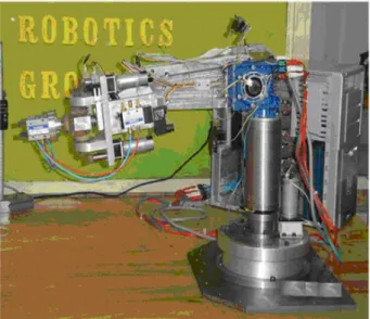
Mobile Robot

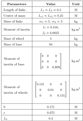
Two-link mobile robot that is used in simulations is shown in Figure 1 and the parameters of this robot are presented in Table 1.

The generalized coordinates are chosen as: q =qb qm=xf yf 0 1 2: (28)

By applying the Lagrange method and computing the position and velocity for each center of mass, the

Figure 1. Two-link mobile robot.

Table 1. Parameters of mobile robot. Parameters Value Unit Length of links L1= L2= 0:5 M

Center of mass Lc1= Lc2= 0:25 M

Mass of links m1= 5, m2= 3 kg

Moment of inertia I1 = 0:416, I2= 0:0625

kg.m2

Mass of wheel 5 kg Mass of base 94 kg

Moment of inertia of base

2 6 6 4

0 0 0 0 0 0 0 0 6:609

3 7 7

5 kg.m2

Moment of inertia of wheels

2 6 6 4

0:131 0 0 0 0:01 0 0 0 0:131

3 7 7

5 kg.m2

b 0.171 M

r 0.075 M

L0 0.4 M

equations of dynamic motion can be written as: 2 6 6 6 6 4 Fx Fy T0 1 2 3 7 7 7 7 5= 2 6 6 6 6 4

J11 J12 J13 J14 J15

J12 J22 J23 J24 J25

J13 J23 J33 J34 J35

J14 J24 J34 J44 J45

J15 J25 J35 J45 J55

3 7 7 7 7 5 2 6 6 6 6 4 xf yf 0 1 2 3 7 7 7 7 5 + 2 6 6 6 6 4 C1 C2 C3 C4 C5 3 7 7 7 7

5: (29)

Also end-eector coordinates are: xe ye =

xf+L1cos(0+1)+L2cos(0+1+2)

yf+L1sin(0+1)+L2sin(0+1+2)

: (30) In this case, the degree of freedom is n = 5 and the end-eector trajectory has m = 2 degrees of freedom. Thus, the redundancy of the system is r = n m = 3. The system has one nonholonomic constraint, according to the motion of the mobile base:

Two other constraints must be applied for redundancy resolution. A pre-dened path is considered for the base, then _xf, _yf, xf and yf can be calculated,

and 0, _0 and 0 are obtained using nonholonomic

constraints.

Using the remaining terms of Equation 29, equa-tions of the system are rewritten as:

1

Sa2

=

J44 J45

J45 J55

1

2

+

R1

R2

; (32)

where:

R1= J14xf+ J24yf+ J340+ C4; (33)

R2= J15xf+ J25yf+ J350+ C5: (34)

6R Fixed Robot

For the second case study, a 6R manipulator as shown in Figure 2, is considered. Also, a schematic view of this manipulator is shown in Figure 3 and Denavit-Hartenberg parameters are demonstrated in Table 2.

Figure 2. 6R conguration [19].

Table 2. Denavit-Hartenberg parameters of 6R. Joint ai (mm) di (mm) i i Related Link

1 36.5 438 -90 1 Link 1

2 251.5 0 0 2 Link 2

3 125 0 0 3 Link 3

4 92 0 90 4 Gripper YAW

5 0 0 -90 5 Gripper PITCH

6 0 152.8 0 6 Gripper ROLL

The transformation matrix, T , is used for forward kinematic computations [21]:

T = 2 6 6 4

nx ox ax px

ny oy ay py

nz oz az pz

0 0 0 1

3 7 7

5 : (35)

The elements of T are:

nx= c6s1s5+ c1(c234c5c6 s234s6);

ny= c234c5c6s1+ c1c6s5 s1s234s6;

nz= c5c6s234 c234s6;

ox= s1s5s6 c1(c6s234+ c234c5s6);

oy= c6s1s234 (c234c5s1+ c1s5)s6;

oz= c234c6+ c5s234s6;

ax= c5s1 c1c234s5;

ay= c1c5 c234s1s5;

az= s234s5;

px= d6c5s1+ c1(a1+ a2c2+ a3c23

+ c234(a4 d6s5));

py = d6c1c5+ s1(a1+ a2c2+ a3c23

+ c234(a4 d6s5));

pz= d1 a2s2 a3s23+ s234( a4+ d6s5): (36)

In these equations, ai and di are shown in Figure 3.

Also si, ci, sijand cijdenote sin(i), cos(i), sin(i+j)

and cos(i+j), respectively. The relation between the

velocity of an end-eector and the angular velocity of joints is expressed by:

V = J _q: (37)

J is the Jacobian matrix of a 6R arm and can be obtained as:

J = 2 6 6 6 6 6 6 4

j11 j12 j13 j14 j15 0

j21 j22 j23 j24 j25 0

0 j32 j33 j34 d6c5s234 0

0 s1 s1 s1 c1s234 j46

0 c1 c1 c1 s1s234 j56

1 0 0 0 c234 s234s5

3 7 7 7 7 7 7 5 ; (38)

Figure 3. 6R schematic conguration.

where:

j11= d6c1c5 s1(a1+a2c2+a3c23+c234(a4 d6s5));

j12= c1(a2s2+ a3s23+ s234(a4 d6s2));

j13= c1(a3s23+ s234(a4 d6s5));

j14= c1s234( a4+ d6s5);

j15= d6c1c234c5+ d6s1s5;

j21= d6s1c5+c1(a1+a2c2+a3c23+c234(a4 d6s5));

j22= s1(a2s2+ a3s23+ s234(a4 d6s5));

j23= s1(a3s23+ s234(a4 d6s5));

j24= s1s234( a4+ d6s5);

j25= d6(c234c5s1+ c1s5);

j32= a2c2 a3c23+ c234( a4+ d6s5);

j33= a3c23+ c234( a4+ d6s5);

j34= c234( a4+ d6s5);

j46= c5s1 c1c234s5;

j56= c1c5 c234s1s5: (39)

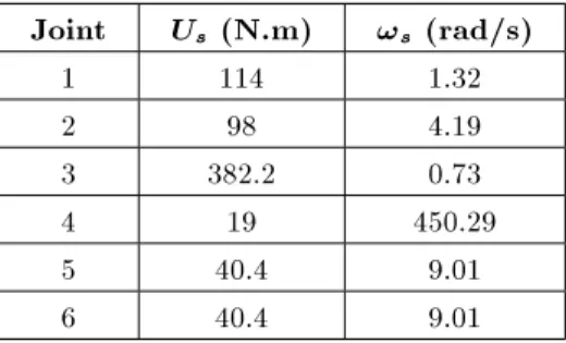
According to Equations 21 and 22, characteristics of motors Usand !sare needed for dynamic load carrying

capacity calculations. These values are determined and collected in Table 3.

Table 3. Motor characteristics for 6R arm. Joint Us(N.m) !s(rad/s)

1 114 1.32 2 98 4.19 3 382.2 0.73 4 19 450.29 5 40.4 9.01 6 40.4 9.01

CONTROL IMPLEMENTATION AND RESULTS

Mobile Robot

For state space representation of a mobile 2-link ma-nipulator, the angular position and velocity of links are chosen as states, as below:

2 6 6 4

1

_1

2

_2

3 7 7 5 =

2 6 6 4

x1

x2

x3

x4

3 7 7

5 : (40)

Thus, the state-space representation is obtained as: d

dt 2 6 6 4

x1

x2

x3

x4

3 7 7 5=

2 6 6 4

x2

P (J55(U1 R1) J45(U2 R2))

x4

P ( J45(U1 R1)+J44(U2 R2))

3 7 7 5 : (41) Parameter P in Equation 41 is:

P = 1

J44J55 J452 : (42)

The predened path for the end-eector is a 1 1 m2

square and the simulation time is 12 sec. At the beginning of the motion, the end-eector is at the left-hand upper corner of this square and point F at the origin. Also, the base moves from the origin to point (2; 0) and then returns to the origin. The actual end-eector paths under full load conditions and upper and lower limits are shown in Figure 4.

The allowable tracking error in Equation 24 is chosen as = 0:02 m and the tracking error is computed according to Equation 23 and plotted in Figure 5. This gure indicates that the maximum error occurred near t = 4 sec at the up side of the square. The angular position and velocity of joints are shown in Figures 6 and 7.

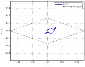
In this case, the ZMP plot shows that stability is guaranteed. For stability consideration, changes in zero moment point location during the motion and limits of stability are shown in Figure 8, where the stability margins are virtual lines between wheels and castor.

Figure 4. End-eector path.

Figure 5. Tracking error.

Figure 6. Angular positions.

Figure 7. Angular velocity of joints.

Figure 8. ZMP and stability margin.

Figure 9 demonstrates the torque of motors and the upper and lower bounds of torques, according to Equations 21 and 22. Using torques and tracking constraints, the dynamic load carrying capacity of manipulator is obtained as 6.1 kg.

6R MANIPULATOR

For the second case study, the vector of state variables for a 6R arm is determined as:

[X]112=

q

_q

: (43)

q is the vector of the angular position of joints:

q =1 2 3 4 5 6: (44)

Also _q is the angular velocities vector:

Figure 9. Torques of motors.

Thus, state-space representation is obtained as: _

X = [x7; x8; x9; x10; x11; x12; D 1(U C G)]: (46)

In Equation 46, D is the inertial matrix, C is the vector of Coriolis and centrifugal forces, G is the gravity force vector and U is the input control vector. Details of these matrix and vectors are as below:

D = 2 6 6 6 6 6 6 4

d11 d12 d13 d14 d15 d16

d12 d22 d23 d24 d25 d26

d13 d23 d33 d34 d35 d36

d14 d24 d34 d44 d45 d46

d15 d25 d35 d45 d55 d56

d16 d26 d36 d46 d56 d66

3 7 7 7 7 7 7 5

; (47)

C =c1 c2 c3 c4 c5 c6T; (48)

G =g1 g2 g3 g4 g5 g6T; (49)

U =u1 u2 u3 u4 u5 u6T: (50)

The control vector is computed through the SDRE method using Equation 20. A linear trajectory is selected for the tracking problem that con-nects initial point P0(0:55; 0:1; 0:5) and nal point

Pf(0:1; 0:3; 0:22) at 10 sec. The line is designed so

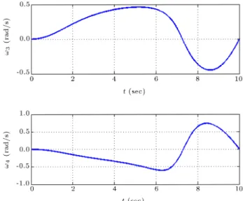
that the velocity and acceleration of the end-eector are zero at both initial and nal points. Actual angular velocities of joints are shown in Figures 10 to 12 for full load conditions. These gures imply that the actual angular velocities of joints are zero at initial and nal points.

Figures 13 to 15 present the actual angular posi-tions of joints under full load condiposi-tions, which indicate a smooth angular motion for joints during the motion. The desired values of angles and angular velocities are computed by solving dierential Equation 37.

Figure 10. Angular velocity of joints 1 and 2.

Figure 11. Angular velocity of joints 3 and 4.

Figure 13. Angular position of joints 1 and 2.

Figure 14. Angular position of joints 3 and 4.

Figure 15. Angular position of joints 5 and 6.

Figure 16. Torques of motors 1 and 2.

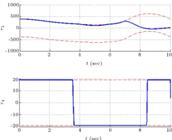
Figure 17. Torques of motors 3 and 4.

The values of torque of each motor are calculated through the SDRE algorithm and are plotted in Fig-ures 16 to 18. The upper and lower values of torques are calculated by Equations 21 and 22 and are shown in these gures. These gures are plotted for maximum load carrying conditions. Moreover, the gures express that the motors work with a maximum value of torque at the beginning of motion.

Conguration links of the manipulator and the actual and desired linear path of the end-eector during the tracking motion are presented in Figure 19, and with a better view in Figure 20.

Tracking accuracy is selected to be = 0:022 m, and according to both limitations on tracking error and motor torques, the dynamic load carrying capacity is obtained as DLCC = 1 kg. Figure 21 illustrates the tracking error as a function of time during the motion. Changes in characteristics of motors and allowable tracking error will aect the value of DLCC.

Figure 18. Torques of motors 5 and 6.

Figure 19. Conguration of robot during tracking.

Figure 20. Desired and actual trajectory

Figure 21. Tracking error.

CONCLUSION

In this paper, the state-dependent Riccati equation is discussed as a nonlinear optimal feedback con-troller. The power series approximation method has been employed for solving the SDRE problem. For a mobile robot, the dynamic load carrying capac-ity with consideration of tracking error and stabilcapac-ity constraint has been obtained. Also, the DLCC of a 6R manipulator is calculated with tracking error consideration. Variations in R and Q matrixes change the value of the tracking error and control eorts. In order to reach better tracking accuracy, elements of matrix R must be decreased, but the period of simulation is increased and the motors come close to saturation conditions. It is seen that the tracking error is appeared as a function of both R and Q, and the tracking accuracy can be increased by changing these matrixes. Dierent state-dependent coecient parameterization, which results in a dierent matrix, A, leads to an additional degree of freedom for the design controller and, as a result, dierent values of DLCC can be calculated. After appropriate state-dependent coecient parameterization, the control design procedure using the SDRE method is systematic and done automatically. It is seen that the SDRE method is suitable for solving nonlinear closed loop optimal control problems and the DLCC can be de-termined using this method for both mobile and xed robotic systems.

NOMENCLATURE

A(x) state-dependent coecient matrix A0 constant part of A(x)

A(x) nonlinear part of A(x) g(x) nonlinear functions in A(x)

f; B nonlinear functions in dynamic equations

J(x) performance index

Q; R states and control weighting matrixes X(x) the solution of SDRE

F base and arm connecting point

L0 the distance from F to the intersection

point of the axis of symmetry with the driving wheel axis

0 the heading angle of platform measured

from X-axis of the world coordinates i the angular displacements of links

i the torques exerted to joints

E tracking error

tracking accuracy

J Jacobian matrix

Jij elements in dynamic equations

jij elements of Jacobian matrix

x vector of state variables x0 initial values of state variables

xzmp; yzmp the coordination of zero moment point

xd; yd; zd desired position of end eector

xf; yf the coordination of F

xe; ye; ze the coordination of E

q the vector of generalized coordinates of the system

qb the vector of mobile base coordinates

qm the vector of manipulator coordinates

T transformation matrix

nx; ny; nz

ox; oy; oz elements of transformation matrix

ax; ay; az

px; py; pz

V velocity vector of end eector

C vector of centrifugal and Coriolis forces

ci elements of C

D inertia matrix of manipulator dij elements of inertia matrix

G gravity force vector

gi elements of G

U input control vector

ui input control torque of links (elements

of U)

Umax; Umin maximum and minimum of motor

torques

Us stall torque of motors

!s no load speed of motor

REFERENCES

1. Korayem, H. and Pilechian, A. \Maximum allowable load of elastic joint robots: Sliding mode control approach", Amirkabir Journal of Science & Technol., 17(65), pp. 75-82 (2007).

2. Korayem, M.H., Davarpanah, F. and Ghariblu, H. \Load carrying capacity of exible joint manipulator with feedback linearization", Int. J. Adv. Manuf. Tech-nol., 29(3-4), pp. 389-397 (2006).

3. Korayem, M.H. and Irani, M. \Maximum dynamic load determination of mobile manipulators via non-linear optimal feedback", Scientia Iranica, Trans. B, Mech. Eng., 17(2), pp. 121-135 (2010).

4. Korayem, M.H., Naja, Kh. and Bamdad, M. \Syn-thesis of cable driven robots dynamic motion with maximum load carrying capacities: iterative linear programming approach", Scientia Iranica, Trans. B, Mech. Eng., 17(3) pp. 229-239 (2010).

5. Korayem, M.H., Firouzy, S. and Heidari, A. \Dynamic load carrying capacity of mobile-base exible-link ma-nipulators feedback linearization control approach", Proceedings of IEEE Int. Conference on Robotics and Biomimetics, pp. 2172-2177 (2007).

6. Korayem, M.H., Heidari, A. and Nikoobin, A. \Maxi-mum allowable dynamic load of exible mobile manip-ulators using nite element approach", Int. J. of Adv. Manuf. Technol., 36, pp. 606-617 (2008).

7. Korayem, M.H., Azimirad, V., Nikoobin, A. and Boroujeni, Z. \Maximum load-carrying capacity of autonomous mobile manipulator in an environment with obstacle considering tip over stability", Int. J. Adv. Manufacturing Technol., 46(5-8), pp. 811-829 (2010).

8. Pearson, J.D. \Approximation methods in optimal control", Journal of Electronics and Control, 13(5), pp. 453-465 (1962).

9. Wernli, A. and Cook, G. \Suboptimal control for the nonlinear quadratic regulator problem", Automatica, 11, pp. 75-84 (1975).

10. Cloutier, J.R. and Cockburn, J.C. \The state-dependent nonlinear regulator with state constraints", American Control Conference, pp. 390-395 (2001). 11. Erdem, E.B. and Alleyne, A.G. \Experimental

real-time SDRE control of an under actuated robot", The 40th IEEE Conference on Design and Control, Florida, pp. 2986-2991 (2001).

12. Innocenti, M., Baralli, F. and Salotti, F. \Manipulator path control using SDRE", Proceedings of the Ameri-can Control Conference, pp. 3348-3352 (2000). 13. Xin, M., Balakrishnan, S.N. and Huang, Z. \Robust

state dependent Riccati equation based robot manipu-lator control", Proceedings of IEEE International Con-ference on Control Applications, pp. 369-374 (2001). 14. Shawky, A., Ordys, A. and Gremble, M.J.

\End-point control of a exible-link manipulator using H-inf nonlinear control via state-dependent Riccati equa-tion", Proceedings of IEEE International Conference on Control Applications, pp. 501-506 (2002).

15. Singh, N.M., Dubey, J. and Laddha, G. \Control of pendulum on a cart with state dependent Riccati equations", Proceedings of World Academy of Science, Engineering and Technology, 3, pp. 676-676 (2008). 16. Cimen, T., State-Dependent Riccati Equation (SDRE)

Control: A Survey, The International Federation of Automatic Control, pp. 3761-3775 (2008).

17. Beikzadeh, H. and Taghirad, H.D. \Nonlinear sense-less speed control of PM synchronous motor via an SDRE observer-controller combination", Proc. of the 4th IEEE Conference on Industrial Electronics and Applications, Xian, China, pp. 3570-3575 (2009). 18. Beeler, S.C., State-Dependent Riccati Equation

Regula-tion of Systems with State and Control Nonlinearities, NASA Langley Research Center, National Institute of Aerospace (2004).

19. Banks, H.T., Lewis, B.M. and Tran, H.T. \Nonlin-ear feedback controllers and compensators: a state-dependent Riccati equation approach", Computational Optimization and Applications, 37(2), pp. 177-218 (2007).

20. Kim, J. and Chung, W.K. \Real time ZMP compen-sation method using null motion for mobile manip-ulator", Proceedings of the IEEE International Con-ference on Robotics and Automation, pp. 1967-1972 (2002).

21. Korayem, M.H. and Heidari, F.S. \Simulation and experiments for a vision-based control of a 6R robot", Int. J. Adv. Manufacturing Technol., 41(3-4), pp. 367-385 (2009).

BIOGRAPHIES

Moharam Habibnejad Korayem was born in Tehran Iran on April 21, 1961. He received his B.S. (Hon) and M.S. in Mechanical Engineering from the Amirkabir University of Technology in 1985 and 1987, respectively. He has obtained his Ph.D. degree

in Mechanical Engineering from the University of Wollongong, Australia, in 1994. He is a Professor in Mechanical Engineering at the Iran University of Science and Technology. He has been involved with teaching and research activities in the robotics areas at the Iran University of Science and Technology for the last 15 years. His research interests includes dy-namics of Elastic Mechanical Manipulators, Trajectory Optimization, Symbolic Modeling, Robotic Multimedia Software, Mobile Robots, Industrial Robotics Stan-dard, Robot Vision, Soccer Robot, and the Analysis of Mechanical Manipulator with Maximum Load Car-rying Capacity. He has published more than 300 papers in international journal and conference in the robotic area.

Mohsen Irani was born in Kashan, Iran on 22 July, 1980. He received his B.S. in Mechanical Engineering from the Isfahan University of Technology in 2002 and M.S. in Aerospace Engineering from the KNTU University of Technology in 2005. He is currently a Ph.D. student in Mechanical Engineering in the Iran University of Science and Technology, Tehran, Iran, since 2007. His research interests includes: Robotic Systems, Nonlinear Control, Optimal Control, Mobile Manipulators, Industrial Automation and Mechatronic Systems.

Saeed Rafee Nekoo was born in Tehran, Iran, on February, 12, 1984. He received the Associate of Me-chanical Engineering from Jabbarian technical Junior College of Hamedan in 2004 and the B.S. in Mechanical Engineering from the Azad University of Tehran, South Branch in 2007. He is presently student of master of Mechanical Engineering in the Iran University of Science and Technology. His current research and interests include: Robotic, Control, Manufacturing, and Mechatronics systems.