Sharif University of Technology
Scientia IranicaTransactions E: Industrial Engineering www.scientiairanica.com
Scaling implementation of a tension rectication
algorithm to solve the feasible dierential problem
M. Ghiyasvand
Department of Mathematics, Faculty of Science, Bu-Ali Sina University, Hamedan, Iran. Received 19 May 2012; received in revised form 16 November 2012; accepted 8 June 2013
KEYWORDS Operations research; Network ows; The feasible dierential problem; Tension rectication algorithm;
Scaling
implementation.
Abstract. The feasible dierential problem is solved using a tension rectication algorithm. In this paper, we present a scaling implementation of a tension rectication algorithm. Let n; m; U denote the number of nodes, number of arcs, and maximum arc capacity value of an arc, respectively. Our implementation runs in O(mn log U), which is O(mn log n) under the similarity assumption. The tension rectication algorithm runs in O(m2) time, so, our implementation is an improvement if n log n < m. Another merit
of our algorithm is that, in cases where the feasible dierential problem does not have a solution, it presents some information that is useful to the modeler in estimating the maximum cost of adjusting the network.
c
2014 Sharif University of Technology. All rights reserved.
1. Introduction
The rst theoretical studies on tension were discussed by Berge and Ghouila-Houri [1,2] at the beginning of the 1960s. In 1971, Pla [3] presented an out of kilter algorithm to solve the minimum cost tension problem. Hajiat [4] showed that Pla's algorithm is not polynomial using a graph family fTn; n 2g on
which it runs necessarily in an exponential number of iterations, namely, 2n+2n 1+2n 2 2 calls to a linear
labeling process. Hamacher [5] developed two pseudo-polynomial time algorithms in 1985: negative cut and shortest augmenting cut algorithms. Other non-polynomial algorithms were given by Rockafellar [6]. Polynomial time algorithms to solve the minimum cost tension problem have been presented by Hadjiat and Maurras [7] and Ghiyasvand [8,9]. Piecewise linear and convex costs of the problem and inverse tension problems have been discussed in [10-14].
Let D = (N; A) be a connected digraph with vertex set, N, containing n vertices, and arc set, A, containing m arcs. We denote an arc from node i to
*. E-mail address: [email protected] (M. Ghiyasvand)
node j by (i; j). Let RA (resp. RN) be a collection of
all ordered m-tuples (resp. n-tuples) of real numbers on set A (resp. N). A vector 2 RAis a tension on graph
G with a potential 2 RN, such that ij = j i, for
each (i; j) 2 A. Each arc, (i; j) 2 A, has a capacity, uij,
that denotes the maximum amount of ijon the arc and
a lower bound lij that denotes the minimum amount
of ij on the arc. Tension is called a feasible tension
if lij ij uij, for each (i; j) 2 A. The feasible
dierential problem determines a feasible tension (if it exists).
A cycle, C, in a directed graph is a sequence i1; i2; : : : ; ik of distinct nodes of N, such that either
(ir ! ir+1) 2 A (a forward arc in C) or (ir+1 !
ir) 2 A (a backward arc in C) for r = 1; 2; : : : ; k (where
we interpret ik+1 as i1). It is obvious that tension is
arc-weighting, having a zero sum on every cycle of the graph, so, for each cycle, C, we have:
X
(i;j)2C+
ij
X
(i;j)2C
ij = 0; (1)
where C+ and C are the forward and backward arcs
d+(C) = X (i;j)2C+
uij
X
(i;j)2C
lij: (2)
The next theorem presents a necessary and sucient condition to conclude that the feasible dierential problem has a feasible tension.
Theorem 1 (Feasible dierential theorem [6, page 193]). The feasible dierential problem has a feasible tension if and only if d+(C) 0 for each cycle,
C.
The feasible dierential problem can be solved using a tension rectication algorithm [6, page 203-5, and 15, page 70]. The tension rectication algorithm runs in O(m2) time ([6], page 205, line 20). When the
feasible dierential problem does not have a feasible tension, this algorithm only computes cycle C with d+(C) < 0.
In this paper, we rst present a scaling idea to solve the feasible dierential problem, then a scaling implementation of the tension rectication algorithm is presented, which is a new method for solving the problem. Our algorithm runs in O (mn log U) time, where U is the maximum arc capacity value of an arc. To avoid systematic underestimation of running time, in comparing two running times, sometimes, it will be assumed that the bound, U, is polynomial bounded in n, namely, U = O(nk), for some constant
k [16]. This assumption is called as the similarity assumption [17, page 60]. Thus, under the similarity assumption [16], our algorithm runs in O(mn log n), which is an improvement if n log n < m (in comparison with the tension rectication algorithm [6,15]).
In cases where the feasible dierential problem does not have a feasible tension, our algorithm not only presents a cycle, C, with d+(C) < 0, but also gives
some information so that the modeler can estimate the maximum cost of repairing the network in order to have a network with a feasible tension.
This paper consists of three sections in addition to the introduction. Section 2 presents a brief outline of the tension rectication algorithm. A scaling im-plementation of the tension rectication algorithm is shown in Section 3. Finally, Section 4 presents a faster implementation of the algorithm described in Section 3. 2. The tension rectication algorithm
In this section, a brief outline of the tension rectica-tion algorithm [6,15] is presented. Given an arbitrary potential, , and its tension , let:
A+= f(i; j) 2 Aj
ij< lijg;
A = f(i; j) 2 Ajij> uijg:
If A+ = = A , tension is feasible. Otherwise
any arc (r; s) 2 A+ [ A is selected. Then, Minty's
Lemma [18] is applied using the following painting of the arcs (i; j) 2 A: red (if lij < ij < uij), black
(if ij lij and ij < uij), white (if ij uij and
ij > lij), and green (if lij = ij = uij). It is obvious
that (r; s) will be black or white.
If the outcome of Minty's lemma is a cycle, C, containing (r; s) terminate; this cycle has d+(C) < 0.
Otherwise, the outcome is a set, W , of nodes, such that (r; s) 2 (W; W ) = f(i; j) j i 2 W , j 62 W g or (r; s) 2 (W ; W ) = f(i; j) j i 62 W , j 2 W g, where W = N W . In this case, the value, , is computed as follows:
= 8 > < > :
uij ij; if (i; j) 2 (W; W );
ij lij; if (i; j) 2 (W ; W );
; otherwise;
where: =
(
lrs rs; if (r; s) 2 A+;
rs urs; if (r; s) 2 A :
Then, the updated potentials are: 0
i =
(
i; if i 2 W;
i+ ; if i 2 W :
The tension rectication algorithm repeats with 0 in
which, after a nite number of iterations, arc (r; s) is nally removed from A+[A . These operations repeat
for each arc in A+[ A and the algorithm can be run
in O(jAj(jA+j + jA j)) O(jAj2) = O(m2) time.
2.1. Application of the feasible dierential problem
The minimum cost tension problem appears in many applications (Rockafellar [6, Chapter 7F]) concerning networks, such as timing of events, location of facilities, shared cost problems, and so on. Let cij denote the
cost on arc (i; j). the minimum cost tension problem determines a feasible tension with minimum cost. The minimum cost tension problem is dened as follows:
min X
(i;j)2A
cijij
s.t. is a feasible tension.
All minimum cost tension algorithms [2-5,7-9,19,20] start with a feasible tension. Thus, before solving the minimum cost tension problem, the feasible dierential problem should be solved in order to nd a feasible tension, or to diagnose that the problem does not have a feasible tension.
3. A scaling implementation of the tension rectication algorithm
In this section, a scaling implementation of the tension rectication algorithm is presented. Given a > 0, we dene tension as a -feasible tension if, for each (i; j) 2 A:
lij < ij < uij+ : (3)
Our algorithm starts out with large and drive toward zero. In each phase, the algorithm tries to nd a -feasible tension using the input 2-feasible tension. The following lemma says that need not start out too big and end up too small.
Theorem 2. = 0 is a (U + 1)-feasible tension. Moreover, if l and u are integer and there exists a -feasible tension , such that 1=m, then, the -feasible dierential problem has a solution.
Proof. By U = maxfjlijj; juijj j for each(i; j) 2 Ag,
we get lij U 0 uij+ U (for each arc i ! j),
which means:
lij (U + 1) < 0 < uij+ (U + 1): (4)
Let = 0, which concludes = 0 is a tension and, by Inequality (4), is a (U + 1)-feasible tension.
Now, considering cycle C, by Eqs. (1) and (2), we get:
d+(C) = X (i;j)2C+
(ij uij) +
X
(i;j)2C
(lij ij):
Tension is -feasible, so, by Inequality (3), we have: d+(C) < X
(i;j)2C+)
+ X
(i;j)2C
m:
Thus, if we have a -feasible tension with 1=m, then, d+(C) > m 1. Since l and u are integer,
d+(C) is integer too, which means d+(C) 0: Cycle C
is arbitrary, so, Theorem 1 concludes that the feasible dierential problem has a solution.
Thus, our algorithm starts with = U and x = 0. In each phase, the input is a 2-feasible tension and the output is a -feasible tension. By Theorem 2, the algorithm runs in O(log(nU)) phases. To explain a phase, we need the following denition.
Denition 1. Given a tension, , for each node, i 2 N, value (i) is dened by the following:
(i) = max 8 > > > < > > > :
lij ij; for each outgoing arc
(i; j) of node i; ri uri; for each incoming arc
(r; i) of node i:
(5) The next conclusion is a result of denitions, which
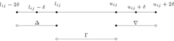
Figure 1. If ij lij, then (i; j) is in the set . If
lij< ij< uij, then (i; j) is in the set . Also, if ij uij,
then (i; j) is in the set r.
Figure 2. If ji> ujior ij< uij, then (i) = (i) [ fjg.
presents a relationship among (i)'s and -feasible tension.
Conclusion 1. Given a tension, . For each i 2 N, (i) < if and only if lij < ij < uij+ , for each
(i; j) 2 A.
Using Conclusion 1, we can work on (i)'s in order to have a -feasible tension. For this purpose, we need the following denitions. Sets r, and are dened in the following way (Figure 1):
= f(i; j) 2 A j lij 2 < xij lijg;
r = f(i; j) 2 A j uij xij < uij+ 2g;
= f(i; j) 2 A j lij < xij < uijg:
Let F () = fi 2 N j (i) < 2g, so, there is a relationship among sets F (); and r, which is as follows.
Conclusion 2. If i 2 F (), then, at least one of the following occurs:
a) There is at least one outgoing arc (i; j) of node i with ij < lij.
b) There is at least one incoming arc (r; i) of node i with ri> uri.
Considering a node i 2 F (), using Conclusion 2, we dene node (i) as follows.
Denition 2. For each outgoing arc (i; j) of node i with ij < lij (resp. incoming arc (r; i) of node i
with ri > uri), let (i) = (i) [ fjg (resp. (i) =
(i) [ frg), see Figure 2(a) and (b).
In each phase of our algorithm, a 2-feasible tension, , should be changed to a -feasible tension, 0.
If F () = , then is -feasible tension, and the current phase is nished. Otherwise, it selects a node, i 2 F (), and labels the nodes using the labeling procedure (i) presented in Algorithm 1. The set of labeled nodes at
Algorithm 1. The labeling procedure.
Algorithm 2. The scaling tension rectication algorithm. the end of the labeling procedure (i) is dened by W .
The following theorem shows how it can be diagnosed when the feasible dierential problem does not have a solution.
Theorem 3. Let W be the set of labeled nodes at the end of the labeling procedure (i). If (i) \ W 6= , then, the feasible dierential problem does not have a solution.
Proof. By the labeling procedure (i), when (i)\W 6= , there is a cycle, C, such that:
(i; j) 2 r; for each (i; j) 2 C+;
(i; j) 2 ; for each (i; j) 2 C : Thus, we get:
X
(i;j)2C+
uij
X
(i;j)2C+
ij; (6)
and:
X
(i;j)2C
ij
X
(i;j)2C
lij: (7)
The arc (i; j) or (j; i) with j 2 (i) is in cycle C, so, by Figure 2, one of Inequalities (5) or (6) is strict. Thus, by Eq. (1), we have:
X
(i;j)2C+
uij
X
(i;j)2C
lij < 0;
which means, using Theorem 1, the feasible dierential problem does not have a solution.
Using Theorem 2 and Conclusion 2, we get the following conclusion, which shows how the feasibility of the feasible dierential problem can be diagnosed. Conclusion 3. If l and u are integer and F () = , such that 1=m, then, the feasible dierential problem has a solution.
Algorithm 2 presents our method, which selects a node, i 2 F (), then removes node i from set F () by
adjusting i' s and ij's, as follows.
0 i=
(
i ; if i 2 W;
i; if i 2 W : (8)
By Eq. (7), ij's are changed according to:
0 ij=
8 > < > :
ij+ ; if (i; j) 2 (W; W );
ij ; if (i; j) 2 (W ; W );
ij; otherwise:
(9) The next lemma proves that node i leaves set F () using Eqs. (7) and (8).
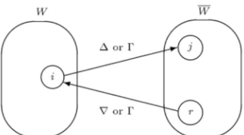
Lemma 1. Suppose that (i) \ W 6= at the end of the labeling procedure (i). After adjusting i' s and ij's,
according to Eqs. (7) and (8), we have (i) < . Proof. Let W = N W . At the end of the labeling procedure (i), we have (Figure 3):
(i; j) 2 r; for each outgoing arc (i; j) of node i with j 2 W ,
(r; i) 2 ; for each incoming arc (r; i) of node i with r 2 W ,
(i; q) 2 or ; for each outgoing arc (i; q) of node i with q 2 W ,
(p; i) 2 r or ; for each incoming arc (p; i) of node i with p 2 W .
We consider the following cases in order to com-pute (i), with regard to 0, computed by Eq. (8):
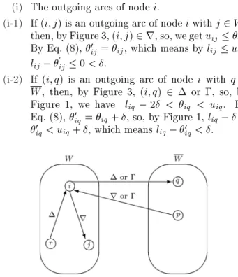
(i) The outgoing arcs of node i.
(i-1) If (i; j) is an outgoing arc of node i with j 2 W , then, by Figure 3, (i; j) 2 r, so, we get uij ij.
By Eq. (8), 0
ij = ij, which means by lij uij,
lij 0ij 0 < .
(i-2) If (i; q) is an outgoing arc of node i with q 2 W , then, by Figure 3, (i; q) 2 or , so, by Figure 1, we have liq 2 < iq < uiq. By
Eq. (8), 0
iq= iq+ , so, by Figure 1, liq <
0
iq< uiq+ , which means liq iq0 < .
Figure 3. After labeling procedure, for each
(i; q) 2 (W; W ), we have (i; q) 2 [ . Also, for each (p; i) 2 (W ; W ), we have (p; i) 2 r [ .
(ii) The incoming arcs of node i.
(ii-1) If (r; i) is an incoming arc of node i with r 2 W , then, by Figure 3, (r; i) 2 , so, we get ri lri.
By Eq. (8), 0
ri= ri, which means, by lri uri,
ri0 uri 0 < .
(ii-2) If (p; i) is an incoming arc of node i with p 2 W , then, by Figure 3, (p; i) 2 r or , so, by Figure 1, we have lpi < pi < upi + 2. By
Eq. (8), 0
pi= pi , so, by Figure 1, lpi <
pi < upi+ , which means pi upi < .
By Denition 1 and cases (i-1),(i-2), (ii-1), and (ii-2), we get (i) < .
Hence, by Lemma 1, node i leaves F (). In order to show that a phase nishes after nite iterations, we prove that the method does not enter a new node to set F ().
Lemma 2. After adjusting i' s and ij's, according
to Eqs. (7) and (8), a new node does not add to set F ().
Proof. By Eq. (8), ij is changed if (i; j) 2 (W; W ) or
(i; j) 2 (W ; W ). Thus, we consider the following two cases:
Case-1. j 2 W with at least oneincoming arc of node j (Figure 4).
Case (1-1). If (i; j) is an incoming arc of node j with i 2 W , then, by Figure 4, (i; j) 2 or , so, we get ij < uij. By Eq. (8), 0ij = ij+ , so ij0 < uij+ ,
which means 0
ij uij < . Thus, by Denition 1, if
node j is not in F (), then, by adjusting ij, according
to Eq. (8), node j will not be added to set F (). Case (1-2). If (j; r) is an outgoing arc of node j with r 2 W , then, by Figure 4, (j; r) 2 r or , so, we get jr > ljr. By Eq. (8), jr0 = jr , so, 0jr > ljr ,
which means ljr jr0 < . Thus, by Denition 1, if
node j is not in F (), then, by adjusting jr according
to Eq. (8), node j will not be added to set F (). Case-2. i 2 W with at least one outgoing arc of node i (Figure 5).
Figure 4. The position of node j 2 W with at least one incoming arc of node j.
Figure 5. The position of node i 2 W with at least one outgoing arc of node i.
Using Figures 3 and 5 and cases (i-2) and (ii-2) in the proof of Lemma 1, if node i is not in F (), then, by adjusting ij's, according to Eq. (8), node i will not
be added to set F ().
The next theorem computes the running time of the algorithm.
Theorem 4. The scaling tension rectication algo-rithm runs in O(mn log(nU)) time.
Proof. Using Theorem 2, the number of phases is O(log(mU)) = O(log(nU)). Each phase, for a given > 0, nishes, if F () = . The algorithm selects a node, i 2 F (), and changes it to (i) < using Eqs. (7) and (8), which takes O(m). By Lemma 2, during a phase, no new node will be added to F (), so, each phase needs jF ()j n iterations. Thus, each phase runs in O(mn).
Now, we show how the information of our algo-rithm is used to estimate maximum cost for repairing the network in order to have a feasible tension. Theorem 5. For a given and i 2 F (), if (i)[W 6= , then, the network can be repaired by, at most, 2m changes in bounds in order to have a feasible tension. Proof. (i) [ W 6= says the feasible dierential problem does not have a feasible tension. Using the method of the algorithm, a 2-feasible tension is computed in the last phase. Thus, we have a tension, , with lij 2 < ij < uij+2 (for each (i; j) 2 A), which
means that m(2) is an upper bound on the number of changes in bounds (increasing uij's or decreasing lij's
by 2), so that be a feasible tension.
4. Reducing the number of phases to O(log U) and nding a feasible tension
At the end of Algorithm 2, we only can diagnose if the feasible dierential problem has a solution, but do not nd a feasible solution. In this section, we reduce the number of phases to O(log U) and compute a feasible solution (if it exists). Let U = 2blogUc+1, so, U >
U + 1, which means, by Theorem 2, = 0 is a U-feasible tension.
Lemma 3. Let l and u be integer. Supposing that the starting is = U, then:
a) If there is a 1-feasible tension, then the feasible dierential problem has a solution.
b) Each 1-feasible tension is a feasible tension. Proof. The starting values are = 2blogUc+1,
ij = 0
(for each (i; j) 2 A), and i = 0 (for each i 2 N).
Thus, initially, is integer and a multiplier of 2. In each iteration, is reduced to =2, which means the values of all 's are integer if 1. During each iteration, the values of i's and ij's are updated by Eqs. (7) and
(8), so, they are integer if 1.
Supposing that we have a 1-feasible tension, , so, lij 1 < ij < uij+ 1, for each (i; j) 2 A. Thus, for
each (i; j) 2 A, we get:
uij ij> 1 ) uij ij 0
(because uij ij is integer);
ij lij > 1 ) ij lij 0
(because ij lij is integer):
Therefore, lij ij uij, for each (i; j) 2 A, which
means each 1-feasible tension is a feasible tension. The next theorem shows that the algorithm can be run in O(mn log U) time using Lemma 3.
Theorem 6. If the scaling tension rectication algo-rithm starts with = U, then, it runs in O(mn log U) time.
Proof. By Lemma 3, each 1-feasible tension is a feasible tension, so, the number of phases is O(log U) = O(log U). By the proof of Theorem 4, each phase runs in O(mn).
Example 1. In this example, we present the imple-mentation of our algorithm for the network in Figure 6. We have U = 5, so, the starting values are =
Figure 6. The network corresponding to Example 1 for applying Algorithm 2.
Figure 7. The initial values for (i)'s and ij's in
Example 1.
2blog5c + 1 = 8, and
i = 0 for each i 2 N (i.e.
ij = 0, for each (i; j) 2 A). The starting (i)'s are
shown in Figure 7: (1) = 0, (2) = 2, (3) = 0, (4) = 1, and (5) = (6) = 1. Hence, we have F (8) = fi 2 N j 8 (i) < 16g = and F (4) = fi 2 N j 4 (i) < 8g = , so, we let = 2 and get F (2) = fi 2 N j 2 (i) < 4g = f2g. For the outgoing arc (2; 6), we have 26 = 0 < l26 = 2,
so (2) = 6 and a labeling procedure (2) should be done, so, we rst label node 2. For the outgoing arc (2; 3), we have 23= 0 = u23, which means (2; 3) 2 r,
so, we label node 3. For the incoming arc (4; 2), we have 42 = 0 < l42 = 1, which means (4; 2) 2 ,
so, we label node 4. Other nodes can not be labeled. We have W = f2; 3; 4g, and W = f1; 5; 6g, so, (2) is not in W . Hence, by Eqs. (7) and (8), we get 2= 3= 4= 0 2 = 2, i= 0 (for other i 2 N),
26 = 0 + 2 = 2, 45 = 0 + 2 = 2, 12 = 0 2 = 2,
64= 0 2 = 2 and ij = 0 for other (i; j) 2 A. The
updated values of (i)'s are (1) = (2) = (3) = 0, (4) = 1 and (5) = (6) = 1.
Now, we have F (2) = fi 2 N j 2 (i) < 4g = , so we let = 1, and get F (1) = fi 2 N j 1 (i) < 2g = f4; 5g. By selecting node 4, updated values of i's
are 2= 3 = 2, 4= 3, 5 = 1 and i = 0 (for
other i 2 N). Updated values ij's are 42 = 56 = 1,
34 = 1, 64 = 3; 26 = 2; 45 = 2, 12 = 2 and
ij = 0, for other (i; j) 2 A. The updated values of
(i)'s are (1) = (2) = (3) = (4) = (6) = 0 and (5) = 1.
Thus, F (1) = fi 2 N j 1 (i) < 2g = f5g. For the incoming arc (4; 5) of node 5, we have 45 =
2 > u45 = 1, so, 4 2 (5) and the labeling procedure
(5) should be done, which gives W = f5; 6; 2; 4; 3g, and (5) \ W 6= . Therefore, the problem does not have a solution. Note, in Cycle C : 5 6 2 4 5, we have d+(C) = (1 + 1) (2 + 1) = 1 < 0.
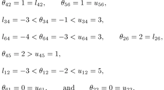
Now, the maximum cost is estimated for repairing this network in order to have a feasible tension. We have F (2) = ;, but F (1) 6= ;. Thus, by Theorem 5, an estimation of the maximum cost of repair is 2m = 2(1)(9) = 18. Of course, we have a lower estimation as follows:
42= 1 = l42; 56= 1 = u56;
l34= 3 < 34= 1 < u34= 3;
l64= 4 < 64= 3 < u64= 3; 26= 2 = l26;
45= 2 > u45= 1;
l12= 3 < 12= 2 < u12= 5;
61= 0 = u61; and 23= 0 = u23:
Thus we only need to change the upper bound arc (4; 5) by 1 unit (i.e. u45should be increased to 2) in order to
repair the network. Acknowledgements
I would like to thank two anonymous referees for their valuable suggestions.
References
1. Berge, C. and Ghouila-Houri, A., Programming, Games and Transportation Networks, Wiley, New York (1962).
2. Ghouila-Houri, A. \Flows and tension in a graph" [Flots et tension dans un graph], Ph.D Thesis, Gauthier-Villars, Paris (1964).
3. Pla, J.M. \An out-of-kilter algorithm for solving mini-mum cost potential problems", Mathematical Program-ming, 1, pp. 275-290 (1971)
4. Hadjiat, M. \Penelope's graph: a hard minimum cost tension instanc", Theoretical Computer Science, 194, pp. 207-218 (1998).
5. Hamacher, H.W. \Min cost tension", Journal of In-formation & Optimization Sciences, 6(3). pp. 285-304 (1985).
6. Rockafeller, R.T., Network Flows and Monotropic Optimization, John Wiley and Sons (1984).
7. Hadjiat, M. and Maurras, J.F. \A strongly polynomial algorithm for the minimum cost tension problem", Discrete Mathematics, 165/166, pp. 377-394 (1997).
8. Ghiyasvand, M. \An O(m(m+nlogn)log(nC))-time al-gorithm to solve the minimum cost tension problem", Theoretical Computer Science, 448, pp. 47-55 (2012).
9. Ghiyasvand, M. \A polynomial-time implementation of Pla's method to solve the MCT problem", Advances in Computational Mathematics and Its Applications, 1(2), pp. 104-109 (2012).
10. Ahuja, R.K., Hochbaum, D.S. and Orlin, J.B. \Solving the convex cost integer dual network ow problem", Management Science, 49, pp. 950-964 (2003).
11. Bachelet, B. and Duhamel, C. \Aggregation approach for the minimum binary cost tension problem", Euro-pean Journal of Operations Research, 197, pp. 837-841 (2009).
12. Bachele, B. and Mahey, P. \Minimum convex-cost tension problems on series-parallel graphs", RAIRO Operation Research, 37(4), pp. 221-234 (2003).
13. Bachele, B. and Mahey, P. \Minimum convex pircewise linear cost tension problem on quasi-k series-parallel graphs", 4OR: Quarterly Journal of European Opera-tions Research Societies, 2(4), pp. 275-291 (2004).
14. Guler, C. \Inverse tension problems and monotropic optimization", WIMA Report (2008).
15. Goh, C.J. and Yang, X.Q., Duality in Optimization and Variational Inequalities, Taylor and Francis, Lon-don (2002).
16. Gabow, H.N. \Scaling algorithms for network prob-lems", Journal of Computer and System Science, 31, pp. 148-168 (1985).
17. Ahuja, R.K. Magnanti, T.L. and Orlin, J.B., Net-work Flows: Theory, Algorithms, and Applications, Prentice-Hall, Englewood Clis, NJ (1993).
18. Minty, G.J. \On the axiomatic foundations of the theo-ries of directed linear graphs", Electrical Networks and Programming, Journal of Mathematics and Mechanics, 15, pp. 485-520 (1966).
19. Hadjiat, M. and Maurras, J.F. \Duality between ow and tension", Actes des Troisiemes Journees du Groupe MODE, Berst, France (1995).
20. Maurras, J.F. \The maximum cost tension problem", Proc. Conf., European chapter on combinatorial opti-mization (ECCO VII), Italy (1994).
Biography
Mehdi Ghiyasvand was born in Hamedan, Iran, in 1975. He obtained his MS and PhD degrees in Operations Research from Tehran University, Iran and spent a post-doctoral term at MIT University, USA. He is now Associate Professor at Bu-Ali Sina University, Hamedan, Iran.