AUSTRALIAN JOURNAL OF BASIC AND
APPLIED SCIENCES
ISSN:1991-8178 EISSN: 2309-8414 Journal home page: www.ajbasweb.com
Open Access Journal
Published BY AENSI Publication
© 2017 AENSI Publisher All rights reserved
This work is licensed under the Creative Commons Attribution International License (CC BY).
http://creativecommons.org/licenses/by/4.0/
To Cite This Article: Showkat Ahmad Bhat and Amandeep Singh., Review on Effective Image Communication Models. Aust. J. Basic & Appl. Sci., 11(8): 65-79, 2017
Review on Effective Image Communication Models
Showkat Ahmad Bhat and Amandeep Singh
Department of Electronics and Communication Engineering, Lovely Professional University, Phagwara, City: Jalandhar, Box: 144401, India.
Assistant Professor Department of Electronics and Communication Engineering, Lovely Professional University, Phagwara, City: Jalandhar, Box: 144401, India.
Address For Correspondence:
Amandeep Singh: Assistant Professor Department of Electronics and Communication Engineering, Lovely Professional University, Phagwara, City: Jalandhar, Box: 144401, India
Phone Number: +919888508706, E-mail: [email protected]
A R T I C L E I N F O A B S T R A C T Article history:
Received 18 February 2017 Accepted 15 May 2017
Available online 18 May 2017
Keywords:
Image, Segmentation, Encoding, Interleaving, Modulation, Fading channels.
Background: Image segmentation is the first stage in image transmission, in which the image is broken into segments. The second stage is encoding where different codes can be used. Interleaving is the third step where block inter-leaver, chaotic inter-leaver are used. The fourth step is modulation where the interleaved data blocks are modulated with the carrier signal. Objective: This paper studies about the different techniques used for efficient image transmission over LTE network under different fading channels. Results: By studying different techniques at each stage of image transmission, the intention is to find the optimum techniques which can enhance the implementation of image transmission over LTE system. The modulation schemes like QPSK, BPSK, and QAM can be used.
INTRODUCTION
LTE is a high-speed wireless communication system for mobile phones and data terminals. Currently, LTE networks have raised themselves to HSDPA technology in order to have high data rates and high capacity for downlink packet data. LTE has attained a data rate of about 100Mbps and about 75 Mbps uplink speed by using HSUPA. LTE uses new modulation schemes for downlink and uplink OFDMA and SC-FDMA respectively. MIMO technology is used for transmitter and receiver antennas which have improved the data rate and efficiency of the LTE. The main requirements of the LTE are high data rate, reduced cost, and more services at low cost, spectrum efficiency, throughput latency, flexible bandwidth, mobility and quality of service. OFDMA is not optimum in the uplink transmission. This is due to the lesser PAPR ratio of the OFDMA in uplink. Thus, both FDD and TDD transmission techniques are supported by SC-FDMA scheme. SC-FDMA has good PAPR ratio in uplink. PAPR ratio is very important in the cost effective design UE power amplifiers. There are certain features of OFDMA similar to SC-FDMA signal operations, so different variables of reverse channel and forward channel can be harmonized. Unlike 3G which is based on circuit switching parallel with the packet switching the LTE (4G) is based on the packet switching only. Packet switching is more desirable than the circuit switching. With the introduction of IPv6, LTE provides higher communication speeds, higher capacity and other diverse usage formats that are compatible with other communication systems. IPv6 is important to support a number of the wireless user equipment. By using IPv6 a large number of addresses is available which overrules the use of Network Address Translation (NAT), a technique of sharing a limited number of IP addresses among a large group of UE’s.
QAM and BPSK for improving Bit Error Rate (BER) and PAPR (peak amplitude power ratio) and Signal to Noise ratio (SNR). Different channel coding, scheduling algorithms, communication channels and channel access schemes are to be used to provide better resource (bandwidth) utilization, Quality of Services (QOS) and to support multiple services, which can achieve by using techniques for data transmission at both the transmitter and receiver ends. Those techniques are selected based on the requirements of the system. There are different types of noises which get added with the information signal and produce errors in the data signal. To enhance the reliability of the LTE network, these errors need to be detected and corrected by the network in adverse conditions.
This paper studies about different techniques to determine the various challenges which occur at every step and which techniques can be used to improve the image transmission through LTE communication system. The complete process of image transmission is described step by step. Section II, proposed image transmission over LTE, section III, image segmentation techniques, section IV, channel encoding techniques, section V, the interleaving schemes, section VI, the modulation schemes and section VII, the fading channels (An Analytical, 2016).
Image Transmission Over Lte:
The processing of image transmission over LTE network is explained by the different stages of the block diagram shown in figure 1. In first step the image is broken into the small data packets by various schemes and then various encoding scheme is applied. Encoding is followed by interleaving process and then different modulation techniques are applied to the encoded data. To transmit data IFFT (Inverse Fast Fourier Transform) is carried out to convert data signal from data domain into frequency domain. And finally is transmitted from the communication channel. At the receiver inverse process as that of transmitter are carried out to receive the original transmitted data. Quality of image is evaluated by measuring the SNR and PSNR. The different transmission stages are studied with details in following section (Kasban1 Mohsen H., et al., 2016).
Fig. 1: Block diagram of image transmission
Image Segmentation:
The pixel sets taken from the original image is able to represent the whole image. Every pixel of the image is assigned a label where pixels with the same label have some common peculiarities. There are different types of image segmentation schemes which are discussed in the following section are edge-based, region-based, Thresh-holding based and clustering based segmentation algorithm (Shi, Y., et al., 2004; YogamangalamInternational, R.,).
A. Edge-Based Segments:
In edge based segmentation the abrupt change in intensity at the boundaries and edges of the image are detected. There are different edge detector operators like Prewitt operator, Sobel operator, and canny operator.
Prewitt Operator:
Prewitt operator is a discrete separation operator, registering a close estimation of the gradient of the image strength per unit. The Prewitt operator provides direction of the most elevated time permits build or diminishing from light with darker. What is the rate of change happening in that specific course by figuring the gradients of the image intensity at each point? The result following applying operator reveals to how "abruptly" alternately "smoothly" those image progress during that side of the point and more in that direction. Also, demonstrates
how probable it will be that and only the image represents to an edge.
(ww.math.washington.edu/~morrow/336_13/papers/debosmit.pdf.).
Mathematically, for ascertaining the close estimation of the derivate the driver convolves the unique image for the 3x3 kernels one to level changes and another for vertical. Though the original image may be characterized Toward A, and Gx and Gy would two images which toward each perspective hold numerous those level and vertical subordinate approximations, the convolutions would be calculated as:
𝐺𝑋= [
−! 0 +1
−1 0 +!
−1 0 +1
] ∗ 𝐴 And 𝐺𝑦= [
−1 −1 −1
0 0 0
+1 +1 +1
]*A (1)
Where * is a convolution operator.
The x-coordinate here indicates the expansion in the up-direction and the y-coordinate in down-direction. At every point, the resultant gradients can be merged together to give the resultant gradient magnitude using:
G = |Gx + Gy| (2)
By utilizing this information, gradient direction can be calculated.
𝜃 = tan 2(𝐺𝑥 𝐺𝑦) (3)
For example, Θ is 0 for a horizontal edge which is darker on the right side.
Sobel Operator:
Sobel operator is a technique for edge detection. It is a discrete differentiation operator, which calculates the approximation of the gradient of the image intensity function. The outcome of this operation is either the standard of the vector alternately the gradient of this vector at each single point.The Sobel–Feldman operator will be in view of convolving those images with a small, separable, and integer-valued channel in both directions (ww.math.washington.edu/~morrow/336_13/papers/debosmit.pdf..
𝐺𝑥 = [
−1 0 +1
−2 0 +2
−1 0 +2
] ∗ 𝐴 𝑎𝑛𝑑 𝐺𝑦= [
+1 +2 +1
0 0 0
−1 −1 −1
]*A (4)
Where * denotes the 2-dimensional convolution operator.
Canny Edge Detection:
Canny edge detection is a process of extracting suitable structural information to reduce the data to be processed from different images. It has been used in different computer vision applications. Thus, an edge identification solution these necessities might make executed for an extensive variety of particular
circumstances (https://www.researchgate.net/publication/228349759;
ww.math.washington.edu/~morrow/336_13/papers/debosmit.pdf). All criteria for edge identification include: 1. Edges are distinguished for low error rate that is edge identification should faultlessly detect large portions edge in those images as possible.
2. From the edge points detected by the canny operator should precisely find the position of the middle point of edge.
3. The edge detected by the canny operator should not be marked more than once, which could create false edges.
1. Apply Gaussian channel filter should smooth birch in the image in place will uproot the commotion (noise).
2. Determine the power gradients of the image.
3. Apply non-maximum concealment on disposing of spurious light of edge identification
4. Apply twofold edge with determine possibility edges.
5. Track edge by hysteresis. Conclude the identification of edges by suppressing every last one of other edges that are feeble which are not associated with solid edges.
B. Thresholding Based Segmentation:
Thresholding is the simplest technique of breaking image into pixel sets by which binary picture is created from grey-level with a black pixel, assuming that the intensity Iij under a threshold value T and with white pixel if the intensity Iij is higher than T. The pixels below certain value are treated as zero and above certain value as one. If f(x, y) is the threshold form of the gray level image h(x, y) towards global threshold value T is shown below.
𝑓(𝑥, 𝑦) = 1, 𝑖𝑓 ℎ(𝑥, 𝑦) > 𝑇
= 0 𝑜𝑡ℎ𝑒𝑟𝑤𝑖𝑠𝑒 (5)
Thresholding operation is represented by 𝑇 = 𝑀[𝑥, 𝑦, 𝑝(𝑥, 𝑦), ℎ(𝑥, 𝑦)] assuming𝑝(𝑥, 𝑦) p(x, y) any point
and ℎ(𝑥, 𝑦)the grey value of that point on the particular image. Based on this there are two methods of threshold
based segmentation. (Different Image Segmentation Techniques, 2014; (IJCSIT) 2014).
Global Threshold:
In global threshold, the value of T solely depend only on the ℎ(𝑥, 𝑦)and T is belong to the characteristics of pixels. The technique is called global threshold.
Local Threshold:
In local threshold, the image is divided into different segments and for each segment, different threshold values are chosen. The value of T depends on ℎ(𝑥, 𝑦) and 𝑝(𝑥, 𝑦). This technique of thresholding is called local threshold.
Utsu Segmentation:
Utsu calculation is generally utilized in light of its effortlessness, furthermore not difficult to utilize. Yet the calculation is main utilized for the 1D image. Utsu algorithm main recognized the grey-level majority of the data without acknowledging those pixel’s spatial neighborhood majority of the data best thereabouts it will be challenging on getting efficient segmentation. This algorithm doesn't work for the points which are widely distributed about center and background change broadly. Utsu segmentation provides for beneficial segmentation impact for two equivalent classes (Different Image Segmentation Techniques, 2014).
C. Clustering Based Segmentation:
Clustering is a process of grouping different image segments having similar characteristics with each other. In this technique, different cluster centers are taken with other neighbor pixels having similar properties one way or the other (Different Image Segmentation Techniques, 2014; (IJCSIT) 2014).
K-means Clustering:
The K-means clustering algorithm determines the data sets (groups) clinched alongside. The information about the dissimilarity between data sets can depend on determining data sets clinched alongside by which cost function of dissimilarities measure is reduced, which is known as the Euclidean distance.
Assume set of n vectors, j =1,....,n , which are divided into c groups G, i = 1,.... c . The object function on the Euclidean distance among a vector Xk in group j and related cluster center Ci can be given by:
𝐽 = ∑𝑐𝑖=1𝐽𝑖= ∑𝑐𝑖=1(∑𝑘,𝑋𝑘 ∈𝐺𝑖‖𝑋𝑘− 𝐶𝑖‖2) (6)
Where, Ji denotes the object function in group i. These different groups are denoted by a Cn binary membership matrix U, here the element Uijis 1 if the jth data point xjis of group i, and 0 otherwise. After selecting and fix the cluster centers Ci, the minimizing Uijfor Equation (1) can be derived as follows:
𝑢𝑖𝑗= 𝑓(𝑥) = {1 𝑖𝑓 ‖𝑋 𝑗 − 𝐶𝑖‖
2
≤ ‖𝑋𝑗 − 𝐶𝑖‖
2
, 𝑓𝑜𝑟 𝑒𝑎𝑐ℎ 𝑘 ≠ 1
0 𝑜𝑡ℎ𝑒𝑟𝑤𝑖𝑠𝑒 (7)
𝐶𝑖 = 1
|𝐺𝑖|∑𝑋𝑘∈𝐺𝑖𝑋𝑘 (8)
Fuzzy C-means Clustering:
Fuzzy C-means clustering (FCM), relies on the concept of k-means clustering, but every data point in Fuzzy is given a membership degree. Fuzzy partitioning is used in FCM, the data points having a value between 1 and 0 of membership function shows the close relationship with several groups. However, FCM still utilizes a cost function, to divide the data sets the cost function has to be decreased. In fuzzy sets membership function (matrix U) can have values between 0 and 1. However, the summation degree of closeness of a data point with all other clusters is always equal to unity (Different Image Segmentation Techniques, 2014; A Comparative Study of Data Clustering).
∑𝑐𝑖=1𝑈𝑖𝑗 = 1, ∀ 𝑗 = 1, …n. (9)
The cost function for FCM is a generalized form of Equation (9):
𝐽(𝑈, 𝑐1, … , 𝑐𝑐) = ∑𝑖=1𝑐 ∑𝑗=1𝑛 𝑢𝑚𝑖𝑗𝑑𝑖𝑗2 (10)
Where the value of uijis in between 0 and 1; Ciis the center of a cluster of fuzzy group i; Euclidean distance in between cluster center and the jth data point is dij= ||c - x||.
The FCM algorithm moves around two states repeatedly until no more change in the result occurs. In a clump mode operation, FCM finds the center of the data groups Ci and the membership matrix U, utilizing those emulating steps:
Step 1: A random variable is used to initialize the membership matrix U between 0 and 1, such that the conditions in equations (1) are fulfilled.
Step 2: Using equation compute the fuzzy cluster centers Ci, i=1...c.
Step 3: Calculate the cost function by using equation (1). Abort if the value of cost function is below a certain threshold value or its improvement is less than in the previous step. Step 4:
Calculate new value of U and go to step 2.
D. Region-Based Segmentation:
Region based segmentation methods are dependent on continuity of certain properties in a particular region of the image. In this technique, the image is divided into different divisions having different characteristics like gray level. Region based techniques depend upon the intensity values of different pixels within a cluster of neighboring pixels. These clusters are called regions, and the objective of this algorithm is to form different groups of these divisions depending upon their functional roles. Region based algorithm is simple compared to edge based segmentation methods and is more immune to noise. Region based segmentation consist of following methods (Region-based Segmentation and Object Detection; Edge Detection Techniques for Image Segmentation).
Region Growing:
Region growing is an operation performed to distinguish the pixels of the image into sub-regions or larger regions according to certain predefined rules. There are four steps in region growing operation:
(i) First, choose a seed pixel set in the original image.
(ii) Define a set of parameters such as gray intensity level or color and define the stopping condition. (iii) Start growing regions by determining the parameters of each neighboring seed with the predefined pixel sets for similarity check.
(iv) Stopthe process when no pixel seems to have similar characteristics based on the predefined rule.
Region Splitting and Merging:
Instead of selecting a seed pixel sets, we can divide an image into various sub-regions and then merge them in order to meet the certain conditions of moderately good image segmentation. Quadtree data is normally used for the implementation of the region splitting and merging image segmentation.
Encoding:
channel problems can cause large distortions. The efficiency of the various channel coding scheme is explained in order to improve the quality of data transmission over the channel (Performance Comparison of Different Forward, 2011; El-Bendary, M.A.M., et al., 2014).
BCH Codes:
BCH is one of the highly effective channel coding scheme among Linear Block Coding schemes. Block size in BCH is given as n=2m-1 and number of check bits in BCH codes are
(𝑛 − 𝑘) ≤ 𝑚𝑡. For any basic integers m and t, there may be a binary (n, k) BCH codes. In BCH coding we
can select different parameters according to our requirement. BCH code is able to correct at a maximumof ‘t’ number of errors. For correcting a single bit error BCH code will work same as Hamming code. BCH codes are most widely used in wireless communication applications. When Signal to Noise ratio (SNR) ids increased in BCH coding BER is minimized almost to zero.
There would three choices provided for of the BCH Encoder block:
(1) Specific Primitive Polynomial: it changes over nonnegative decimal basic d on a binary row vector. The output d vector comes out in matrix form, whose each row is the binary value of the corresponding element value in vector d.
2) Specific Generator Polynomial: a generator polynomial utilizing Galois column vector that schedules those polynomial's coefficients in decreasing order of the variable.
3) Puncture Code: when there are different codewords per frame and are given to encoder, all code words are operated with some puncture pattern. The function of Puncture code word is to discard the parity symbol from code words.
There would be two steps in BCH decoder:
1) If receiver at the input port generates erasures, the performance of the BCH decoder is enhanced especially in fading channel.
2) Output number of error-corrected: it indicates how many detected errors are corrected at the output.
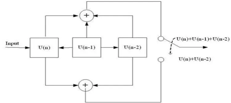
Convolution Encoder:
Convolution codes generate the parity bits by sliding application of Boolean polynomial to detect and correct the error in a data stream. Convolution of encoder over data is done by the application of sliding window. Three parameters are used for the representation of convolution codes n K, h where k denotes how many shift registers used in the encoding block. In convolution codes the continuous stream of data is used at the encoder's input. The codes obtained after encoding also depend on the previous information bits transmitted and the k bit information message. Convolution codes are used in random errors. Convolution codes with block codes are used to increase their performance. In Fig. 2 below, convolutional encoder is shown having the constraint length 3 and has ½ data rate due to two adders used in it. At LSB the bit is shifted towards left and bits at MSB are shifted towards right. Then afterward applying the modulo-2 operation relating outputs requirement. This process is continued until the data reaches at the input port of encoder. The characteristics of code depend on how the shift registers are connected with each other (El-Bendary, M.A.M., et al., 2014).
Turbo coding:
Turbo coding is iterated soft computing method of producing block codes deduced by combining more than one convolution codes with an interleaving that can operate in a fraction of a decibel of Shannon limit. Shannon coding can be achieved by using large block lengths codes, but due to the large requirement of processing power makes it impossible. Turbo codes remove these drawbacks by using recursive coders. Recursive coders make the short length codes to appear block codes and soft decoder improves the reception of messages.
A simple type of convolutional coder can generate turbo codes. The coder is shown in figure (3a) having certain inputs and a constraint length K=3. Multiplexing the outputs produces a code of rate R=1/2.
Fig. 3: Convolution coder
The convolutional coder shown in figure (1b) is called recursive convolutional coder in which one of the outputs p0 has been given feedback at the input port make it recursive.
Low-density parity-check (LDPC) codes:
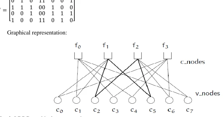
LDPC code corrects the linear block errors code and is used for transmitting data over a very high noisy channel. The sparse bipartite graph is used for the generation of low-density parity codes. LDPC codes are capacity dependent codes and can be constructed practically by keeping the noise threshold value near to the theoretical maximum for the symmetricalmemoryless channel. By setting the noise threshold, we select the upper bound for the channel noise, where the probability of data loss can be made possible. Using iterative belief propagation techniques, LDPC codes are represented by matrices and graphical representation. Let’s look at the examples of matrices and the graphical representation is shown below (Chan, F. and D. Haccoun, 1997):
Matrices representation:
𝐻 = [ 0 1 1 1
0 1 1 0 0 0 1 0
1 0 0 1
1 0
0 1
0 1
0 0
0 1
1 0
1 1
1 0
] (11)
Graphical representation:
LDPC code algorithm:
The steps of the algorithm are given below:
1. The V node is given a received code word value.
2. The value from V node is transported to each of the connected C nodes. 3. The value of an edge is computed in C-nodes and transmitted back to V node.
4. The value received from C node is added with original code word value and the values are updated. 5. Steps 2 – 4 are repeated for a predefined number of iterations.
6. The final values are calculated at V nodes and the values are corrected results.
Fig. 5: Block diagram of LDPC encoder and decoder
Hamming code:
Hamming codes are linear error correcting code and are used for detection of a single bit and two bits errors. Hamming codes are suited for random errors, not for errors that come in bursts. With contrast to the parity, codes cannot correct errors and are able to detect only odd error bits in errors. Hamming codes are very accurate codes and having a high rate of codes with block length and minimum distance.
Mathematically, Hamming codes are the class of binary linear codes. Hamming codes are shortened Hadamard codes. To each integer r ≥ 2, there may be a code for square length n = 2r −1 What's more message length k = 2r − r − 1. Consequently, those rate from claiming hamming codes is r = k / n = 1 − r / (2r − 1), which is the minimum achievable for codes with least separation of three and block length 2r − 1. Block diagram of
Hamming code encoder and decoder is given in figure 6:
Interleaving:
Interleaving is a process or methodology of rearranging the data in non-contiguous manner to make system more reliable, efficient and fast based on predefined rules. To receive the data at receiver side the reverse rule is followed to retrieve the original data symbols. Interleaving of the binary data is important before modulation because it allows long distance propagations in different difficult propagation conditions. There are different interleaving techniques (Shi, Y., et al., 2004; (IJAIEM)).
Block Interleaver:
Without repeating or omitting any elements the block Interleaver rearranges the elements of input. The input to the block interleaver can be any number (real or imaginary). If there are N elements at input, the element parameters are given by a vector of length N. Square Interleaver rearranges those components for its information without rehashing decimal alternately omitting At whatever components. That information might a chance to be genuine or mind boggling. If those information holds n elements, that point the components parameter will be a vector from claiming period n that demonstrates those indices, to order, of the enter components that manifestation the length-N yield vector. Block Interleaver may be basic and simple should execute over different systems. A block interleaver will be in the structure of a row-column grid from claiming size RxC; the place R may be aggregate number of rows C’s may be those downright number from claiming columns. To perform interleaving, the majority of the data may be composed of the RxC row-column grid can be read back in column wise as shown in figure (7). There would no inter-row or inter-column permutations utilized within this illustration, consequently those interleaved arrangement holds a percentage precise request. The piece de-interleaver performs the opposite operation of the interleaver over which the data is composed of the RxC row-column grid section insightful Also perused over to column insightful.
Fig. 7: Block Interleaving
Convolution Interleaver:
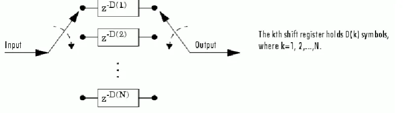
Convolutional interleaver consists of shift registers, each register having a fixed delay. The delays in a conventional convolutional interleaver are a non-negative integer multiple of a fixed integer. The new symbols are added to the next register from the input and the previous data symbols from that register go in the output vector. The functioning of interleaver depends upon the past symbols along with current symbols feed oninput, that is a convolutional interleaver requires memory for its operation. A schematic diagram (8) and below explain the structural block diagram of the convolutional interleaver having some shift registers with delay values D(1), D(2)...,D(N). The blocks in this library have hidden parameters that show the delay of every shift register. The convolutional encoder and decoder are shown in figure (9).
Fig. 9: Convolutional interleaver and deinterleaver
When an arranged data is passed through a convolutional interleaver and an comparing deinterleaver, the detected data lags behind those first succession data. The delay between the original and restored sequence is (Number of shift registers)*(Maximum delay among all shift registers) for the most general multiplexed interleaver.If there incurs an extra delay between interleaver outputs and deinterleaver input, that point those restored data arrangement lags behind first grouping. Eventually, this aggregates the extra delay and the add up in the first equation.
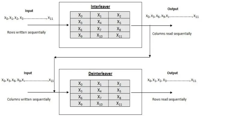
Matrix interleaver:
Matrix interleaver is also a block interleaver. This process is done by feeding the data into matrix rows by row and output is given by matrix interleaver at output column by column. The dimensions of the matrix are determined by the number of rows and columns which are used for block computation. Matrix interleaver shown in figure (10) is a block interleaver in which that data is fed into matrix row by row and retrieved at output column by column. The deinterleaver performs deinterleaving operation by feeding the matrix with the input data sequence column by column and reverse operation at output. The input vector length must be equal to Number of rows times Number of columns.
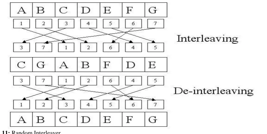
Random interleaver:
Random interleaver block performs interleaving by using a random permutation to rearrange the components of its input vector. The number of elements present in the input vector denotes how many element parameters are there. A column vector is utilized if the input data is in frames. Random interleaver Figure (11) rearranges the input data before sending it into the channel with various predefined permutation schemes. Because of this random arrangement of data, the error symbols gets randomizer at the receiver side. After the randomization of the error bursts, due to which the whole data blocks gets rearranged and can now be detected and corrected easily.
At interleaverside, pseudo-random permutation is generated of available memory addresses. The data symbols are rearranged according to these generated pseudo-random orders of memory addresses. The data can be received and interleaved at deinterleaver side only if it knows the exact order of permuter-indices. The de-interleaver should know the order of pseudo codes exactly as that in de-interleaver.
Modulation:
Modulation is a process of mapping the code bits in a format that is effectively sent over the communication channel. A modulation scheme converts the digital data signal into the signal which can be transmitted through the communication channel. The main aim of the modulation is to compress the data as much as possible into the spectrum or bandwidth available. There are different techniques of modulation (Comparison of Different Digital Modulation Techniques 2016; BPSK and QPSK).
Fig. 11: Random Interleaver
Quadrature amplitude modulation (QAM):
QAM is used for both analog and digital modulation. It carries only two message signals whether those are analog or two digital bit streams, by modulating (changing) the amplitude of carrier waves by using amplitude shift keying (ASK) digital modulation scheme or amplitude modulation (AM) analog modulation scheme. The carrier waves are of the same frequency but are out of phase by 90 degrees from each other and are called Quadrature components. QAM is most widely used modulation scheme in telecommunication systems. The QAM modulator block diagram is shown in figure 1. By using QAM the high bandwidth utilization can be achieved by selecting suitable constellation size which is limited by noise and linearity of the channel. On the transmitter side of QAM modulator, the modulated QAM wave is of the form (Comparison of Different Digital Modulation Techniques 2016).
𝑆(𝑡) = 𝑅𝑒{[𝐼(𝑡) + 𝑖𝑄(𝑡)]𝑒𝑖2𝜋𝑓𝑜𝑡}
= cos(2𝜋𝑓𝑜𝑡) − 𝑄(𝑡) sin(2𝜋𝑓𝑜𝑡) (12)
Where 𝑄(𝑡) is Quadrature components and 𝐼(𝑡) is in-phase and components, f0 is the carrier frequency and
𝑅𝑒{ } denotes real part.
At the demodulation side the 𝐼(𝑡)and 𝑄(𝑡)components can be detected separately by multiplying them with
cos(𝑡) and sin(𝑡) respectively and the expression is of the form
𝑟(𝑡) =1
2𝐼(𝑡)[1 + cos(4𝜋𝑓𝑜𝑡)] −
1
2𝑄(𝑡) sin(4𝜋𝑓0𝑡) (13)
Quadrature Phase Shift Keying:
In QPSK two such sinusoidal signals (sine and cosine) are chosen as basic functions for modulation of the original baseband signal. In QPSK the modulation is done by changing the phase of the sinusoidal basis functions with respect to the message symbols. In QPSK one symbol represents two bits as it is the symbol based modulation scheme. The mathematical equations of QPSK modulation scheme is of the form
Si (t) = 2𝐸𝑠T-√cos (2π𝑓0t+ (2n−1)4𝜋), n=1, 2, 3, 4 (14)
The phase shift takes different values by changing the values of integer n, phase shifts can be of 450 and are called Pi/4 QPSK. Thus QPSK modulation signal consists of in-phase (I) and Quadrature component (Q).
A QPSK modulator block diagram is shown in figure (12) below. A serial to parallel converter (de-multiplexer) is used to discriminate between the even and odd bits from the data bits produced by thegenerator. Each single odd bits and even bits are converted to NRZ format. I-arm and Q-arm are applied to multipliers and multiplied by cosine and sine components respectively and then adding the resultant signal I-arm and Q-arm to generate QPSK modulated signal.
Fig. 12: QPSK Modulator
For coherent demodulation of QPSK signal, the demodulator must know at what carrier frequency and phase the signal is modulated prior to perform demodulation.
BPSK Modulation:
Binary phase shift keying is used for low data rate applications. BPSK can modulate one symbol per symbol then it is unsuitable for high data rate applications. Binary phase shift keying (BPSK) is a low data rate modulation technique which sends only one bit per symbol i.e., 0 and 1. BPSK has same bit rate and symbol rate as we are sending only one bit per symbol. We can have a phase shift of 0 degrees or 180 degrees with respect to a reference carrier depending upon the message bit. The BPSK band pass signals are of the form given below.
𝑆1= √
2𝐸
𝑇 cos(2𝜋𝑓𝑡) → 𝑟𝑒𝑝𝑟𝑒𝑠𝑒𝑛𝑡𝑠 ′1′ (16)
𝑆2= √
2𝐸
𝑇 cos(2𝜋𝑓𝑡 + 𝜋) → 𝑟𝑒𝑝𝑟𝑒𝑠𝑒𝑛𝑡𝑠 ′0′
𝑆2= −√
2𝐸
𝑇 cos(2𝜋𝑓𝑡) → 𝑟𝑒𝑝𝑟𝑒𝑠𝑒𝑛𝑡𝑠 ′0′ (17)
Where E is the symbol energy, T denotes time period and f represents the carrier frequency.
Fading channel models:
In mobile communication systems, the signals can travel from source to destination through different reflected paths, which introduces the multipath fading; transmitted signal can travel from multiple reflected paths from the transmitter to the receiver, due to which channel fading, attenuation, amplitude variations, phase and angle variations. Fading can be defined as the variation of the attenuation of a signal with different variables. Fading channel models are used for determining the effects of this fading accurately on the signal in order to decrease its effects. Fading are used for the simulation of the errors in wireless communication. AWGN, Rayleigh, and Racing are the most widely used fading models (BER).
AWGN channel:
noise-like thermal noise, shot noise, black body radiation and from manmade sources. The Central limit theorem of probability theory shows that AWGN has Gaussian or normal distribution. AWGN channel is used for analyses of modulation techniques when noise is added with signal passing through AWGN channel. AWGN has flat frequency response and linear phase response for all frequencies. AWGN does not introduce any phase distortion and amplitude loss to the signals passing through it. So in such cases, fading is not present but distortion is introduced by the AWGN channel. The signal at the receiver is simplified𝑟(𝑡) = 𝑥(𝑡) + 𝑛(𝑡). Where n (t) denotes the added noise (PSK System, 2012).
Racian Fading Channel:
Racian fading is a stochastic model for a signaltraveling through channel deviations occur by partial cancellation of the signal by itself. The radio signal travels to the receiver station through multiple paths and some paths are always changing. Racian fading happens because of high energy signals received through a direct path, stronger than other signals. In Racian fading, the amplitude gain is characterized by a Racing probability distribution. Signals’ traveling from the direct line of sight paths are strongest and faces more fading than multipath components. These types of signals are approximated by Racian distribution (Nassar, S., et al., 2016).
𝑝(𝑟) = 𝑟
𝜎2𝑒
−(𝑟2+𝐴2
2𝜎2 )𝐼 (𝐴𝑟
𝜎2) 𝑓𝑜𝑟 (𝐴 ≥ 0, 𝑟 ≥ 0) (18)
Where A is peak amplitude of dominating signal and I ( ) is the zero order modified Bessel functions.
Rayleigh Fading Channel:
Rayleigh fading channel is statistical model used for estimating the impact of propagation channel on a radio signal usually used for wireless communication. In this model, we consider that amplitude of signal passing through channel will remain varying randomly of fade.Rayleigh channel model will be viewed as effective to tropospheric What's more ionospheric too to urban surroundings sign proliferation. Rayleigh model is used when there is no direct communication path between transmitter and receiver stations (Nassar, S., et al., 2016). Rayleigh model is special case of “two wave with diffuse power” (TWDP) fading. Rayleigh is used when there is high density of objects that scatter the radio signals before reaching the receiver. If there will be no predominant part in the scatter, those processes are having zero mean and phase uniformly divided between 0 and 2π radians. The channel will therefore be characterized by Rayleigh distribution. The probability density function of Rayleigh channel is given by Rayleigh channel is given by
𝑃 𝑟𝑎𝑦𝑙𝑒𝑖𝑔ℎ(𝑟) = 𝑟
𝜎2 𝑒𝑥𝑝 (−
𝑟2
2𝜎) (19)
Where 𝜎 standard deviation and r is random variable. The main source of Rayleigh noise is due to the multipath propagation of signals from transmitter to the receiver and when there is no line of sight communication channel available between transmitter and receiver.
Fig. 14: Flow chart of image transmission
Conclusion:
The objective of this paper is to study the optimum technique at each stage to obtain optimum performance of the image transmission over LTE network under Rayleigh fading channels. Rayleigh fading channel can be used for multipath propagation having no line of sight communication between transmitter and receiver stations and can be used for LTE in heavily built up areas. From all the segmentation techniques, Threshold-based segmentation is the best segmentation technique which gives accurate results and is computationally fast. At encoding stage, RS-CC (Reed Solomon-Convolutional codes) codes have good burst error correcting capability and have low BER. AT interleaving stage convolutional interleaving is used because it is more efficient and has less BER rate. For modulating the data signal, QAM modulation is capable to transmit more bits per symbol and large data can be transmitted over small bandwidth and also has low BER. Figure (12) shows the complete image transmission using these efficient techniques at each stage. Using these techniques at each stage, optimum or high performance image transmission can be obtained.
REFRENCES
Kasban1 Mohsen H., A.M. Mohamed Kaseem El-Bendary2, 2016. Performance Improvement of Digital Image Transmission over Mobile WiMAX Networks, Springer Science-Business Media.
An Analytical, 2016. Approach to Improve the Performance of Image Transmission over Mobile WiMAX NetworksInternational Journal of Advanced Trends in Engineering, Science, and Technology(IJATEST) 4: 1.
A Study Analysis on the Different Image Segmentation Techniques, 2014. International Journal of Information & Computation Technology. ISSN 0974-2239 4(14): 1445-1452.
A Review on Otsu Image Segmentation Algorithm, 2013. International Journal of Advanced Research in Computer Engineering & Technology (IJARCET) 2: 2.
Edge Detection Techniques for Image Segmentation - A Survey of Soft Computing Approaches, research gate November 2007, https://www.researchgate.net/publication/228349759.
Comparison of Different Digital Modulation Techniques 2016. in LTE System using OFDM AWGN Channel, International Journal of Computer Applications (0975 – 8887) 143: 3.
YogamangalamInternational, R., Journal of Engineering and Technology (IJET), Segmentation Techniques Comparison in Image Processing.
Shi, Y., X.M. Zhang, Z.C. Ni and N. Ansari, 2004. Interleaving for combating bursts of errors. IEEE Circuits and Systems Magazine, 4: 29-42.
Gallager, R., 1962. Low-density parity-check codes. IRE Transactions on information theory, 8(1): 21-28. Chan, F. and D. Haccoun, 1997. Adaptive Viterbi decoding of convolutional codes over memory less channels. IEEE Transactions on Communications, 45(11): 1389-1400.
Nassar, S., N.M. Ayad, H.M. Kelash, H.S. El-Sayed, M.A.M. El-Bendary, F.E. Abd El-Sammy et al., 2016.
Content verification of encrypted images transmitted over wireless AWGN channels. Wireless Personal Communications
El-Bendary, M.A.M., H. Kasban and M.A.R. El-Tokhy, 2014. Interleaved reed-Solomon codes with code rate switching over wireless communications channels. In: International Journal of Information Technology and Computer Science (IJITCS).
Image Performance over AWGN Channel Using PSK System, 2012. International Journal of Engineering and Innovative Technology (IJEIT) 2: 1.
Design and Implementation of Area Efficient BPSK and QPSK Modulators Based On FPGA.
Implementation of Different Interleaving Techniques for Performance Evaluation of CDMA System. International Journal of Application or Innovation in Engineering & Management (IJAIEM).
BER Performance of Digital Modulation Schemes With and Without OFDM Model for AWGN, Rayleigh and Racian Channels.
4th Generation (4G) Technological Infrastructure and Enhanced Mobile Learning: An Effective Tool for Open and Distance Education.
Edge Detection Techniques for Image Segmentation – A Survey of Soft Computing Approaches N. Senthilkumaran1 and R. Rajesh.
Review: Various Image Segmentation Techniques, 2014. Swati Matta / (IJCSIT) International Journal of Computer Science and Information Technologies, 5(6): 7536-7539
Edge Detection in Digital Image Processing Debosmit Ray, Thursday, June 06, 2013. ww.math.washington.edu/~morrow/336_13/papers/debosmit.pdf.
Some refinements of rough k-means clustering, Georg Peters, Department of Computer Science/Mathematics, Munich University of Applied Sciences, Lothstrasse 34, 80335 Munich, Germany.
A Comparative Study of Data Clustering, Techniques, Khaled Hammouda Prof. Fakhruddine Karray University of Waterloo, Ontario, Canada.
Region-based Segmentation and Object Detection, Stephen Gould1 Tianshi Gao1 Daphne Koller2 1 Department of Electrical Engineering, Stanford University.
An Introduction to Turbo Codes Matthew C. Valenti1 Bradley Dept. of Elect. Eng., Virginia Polytechnic Inst. & S.U., Blacksburg, Virginia.