Journal of Industrial and Systems Engineering
Vol. 8, No. 3, pp 42-58 Summer 2015
Multi-objective robust optimization model for social responsible
closed-loop supply chain solved by non-dominated sorting genetic
algorithm
Hamid Saffari
1, Ahmad Makui
2*, Vahid Mahmoodian
3, Mir Saman Pishvaee
4 1-4 School of Industrial Engineering, Iran University of Science and Technology, Tehran, Iran.[email protected], [email protected], [email protected] [email protected]
Abstract
In this article a supply chain network design model has been developed considering both forward and reverse flows through the supply chain. Total Cost, environmental factors such as CO2 emission, and social factors such as employment and fairness in providing job opportunities are considered in three separate objective functions. The model seeks to optimize the facility location problem along with determining network flows, type of technology, and capacity of manufacturers. Since the customer’s demand is tainted with high degree of uncertainty, a robust optimization approach is proposed to deal with this important issue. An efficient genetic algorithm is applied to determine the Pareto optimal solutions. Finally, a case study is conducted on a steel industry to evaluate the efficiency of the developed model and its solution algorithm.
Keywords: supply chain; reverse logistic; social responsibility; robust optimization; multi-objective genetic algorithm.
1-Introduction
Closed loop supply chain problems consider facility location and allocation along with forward and reverse flows of materials and goods are optimized. Forward logistics investigate all the processes for delivering goods to the end customers. On the other hand, reverse logistics is related to the processes of gathering used products and making decision about recycling or discarding them. There is another case in which both forward and reverse flows are being considered simultaneously.
In the last two decades, design of logistic networks considering both forward and reverse flows has grown due to resource constrains, increased costs and consequences of utilizing new products instead of used products on environment. A rise in environmental contamination challenges such as greenhouse gases emission, necessity to consider human rights and collecting of returned products have encouraged governments to consider determining new controlling rules and as a result, different standards such as ISO 26000 (2006) have been developed. Standard ISO 26000 considers social responsibility concepts and issues, and provides an approach to integrate social responsibility with solutions, systems and current organizational activities.
*Corresponding author.
In real world, insufficiencies and inaccuracies in data can result uncertainties in designing an appropriate supply chain. To cope with uncertainties, robust programming approach has taken into consideration, since mean value of variables or other common approaches in literature do not provide a suitable representative of real world (Mulvey et al., 1995).
In most of the articles related to supply chain design, only profits and costs have considered to be optimized. Growing concern on environmental issues such as greenhouse gases emission and global warmth on one hand, and considering social responsibility issues in organizations, standards like ISO 26000 and other government disciplines on the other hand have influenced organizations to consider environmental issues and social responsibilities such as creating job opportunities and social development along with minimizing costs.
In this paper, a mixed integer programming model have been developed for supply chain design considering forward and reverse flows and factors such as social, economic and environmental issues. In addition, robust programming approach proposed by Mulvey et al. (1995) has been applied due to demand uncertainty. Apart from that a multi-objective genetic algorithm has been developed to solve the model and extract Pareto frontier.
The rest of the paper has been organized as follows. The literature of the scope has been reviewed in section 2. Robust optimization is described in section 3. Problem definition and mathematical modeling for deterministic and non-deterministic conditions are included in sections 4 and 5. The description of solution method is presented in section 6 and section 7 contains application of model on a real case. Finally, concluding remarks are given in section 8.
2- Literature review
2-1- Proposed supply chain models considering forward and reverse flows
Fleischmann et al. (2001) proposed a general facility locating problem which was one of the pioneer studies to consider forward and reverse flow at the same time. Sim et al. (2004) developed a multi-product, multi-period model with constraints in numbers and capacities of facilities. In their work, different transportation modes like marine transportation, road transportation, air and train transportation was considered and the model was solved with genetic algorithm.
Salema et al. (2005) also developed a supply chain model considering forward and reverse logistics. They have considered two periods. Decision making for facility locations happens in longer period and network flows decision making has been considered in short period. Their mathematical model was solved with branch and bound algorithm and a scenario-based approach was applied to include uncertainty. Salema et al. (2007) provided uncertainty of demand and return rate in their model using scenario generation, too.
Ko and Evans (2007) presented a mixed integer non-linear programming model for third party organizations and utilized genetic algorithm to solve the model. Lee and Dong (2007) addressed a two stage solution method and a tabu search meta-heuristic approach to deal with forward and reverse flows of computer products supply chain. Wang et al., (2010) developed a model for forward/ reverse logistics and applied a genetic algorithm based on spanning tree approach to solve the model.
Pishvaee et al. (2009) proposed a scenario based optimization model for closed loop supply chain design. In their work, demand, transportation costs, numbers of returned products, and quality of returned products were considered as uncertain parameters. Easwaran and Üster (2010) presented a model for closed loop supply chain and used Benders’ decomposition method to solve it. El-Sayed et al. (2010) developed a product multi-echelon multi-period model. They also included risk in their study.
Pishvaee and torabi (2010) addressed a fuzzy bi-objective mixed integer programming model with objective functions of cost minimization and customer response maximization for a supply chain design. The model was solved with a possibilistic fuzzy approach. In another study by Pishvaee et al. (2010) a bi-objective model was developed and solved with a heuristic algorithm. A robust programming approach was applied for forward and reverse flow logistics by Pishvaee et al. (2011) for the first time.
Das and Chowdhury (2012) developed a model for closed loop supply chain. They assumed that collected products have different quality levels and returned products can be recycled. Özkır and Başlıgil (2012) presented a mixed integer programming model for closed supply chain design and determined three options for recycling returned products; material recycling, component recycling, and product recycling.
Vahdani et al. (2013) developed a novel model considering reliability for closed loop network design. They considered failure probability for each collection center and used robust optimization model and queuing theory to cope with uncertainty. Hassani et al. (2012) addressed a supply chain design with uncertainty in demand and also purchasing costs. They considered robust programming approach and used Bill of Material (BOM) for new and returned products. Rosa et al. (2013) developed a robust model to minimize the regret of different scenarios and included uncertainty by log-normal distribution. They also considered three categories of small, medium and large warehouses and determined their optimum capacity.
Özkır and Başlıgil (2013) presented a multi-objective model for maximizing satisfaction level of trade, customer response, and profit. They used fuzzy numbers to include uncertain parameters in their model.
Ramezani et al. (2013a) developed a model for supply chain design to optimize forward and reverse flows. They defined three objective functions to optimize the profit, the service level both in forward and reverse logistics, and poor quality materials sent from supplier. Ramezani et al. (2013b) also developed another single objective model and used minimizing the maximum regret level rather than taking the average of different scenarios. They also introduced an algorithm to create different scenarios.
Subramanian et al. (2013) presented a mixed integer programming model to determine optimum locations of plants, distribution centers, recycling centers and disposal centers, and to optimize material flows among these facilities. They used simulated annealing meta-heuristic approach to solve their model.
Keyvanshokooh et al. (2013) considered both pricing and forward and reverse supply chain design and in their model, each customer decided about returning used products based on the proposed price. They also assumed that the products can be transferred inside one echelon of supply chain. The studies which considered environmental and social issues are investigated in the following as well.
2-2- Papers considering environmental issues
Amin and Zhang (2013) presented a multi-product bi-objective model considering cost and use of environmental friendly material in a closed loop supply chain. They employed weighted sum method and ɛ-constraint method to solve their model. Pishvaee and Razmi (2013) addressed a fuzzy programming model and considered environmental effects as their second objective function. Wang et al. (2012) developed a multi-objective model for minimizing cost, CO2 emission and waste. The model was also proposed to determine optimum locations of plant of new and remanufactured products, distribution centers, and recycling centers along with optimum flows among facilities.
2-3-
Papers considering social issues
Cartend and Jennings (2002) surveyed social effects of purchasing on supply chain performance and showed that the purchasing based on social criteria has direct and positive impacts on suppliers performance. They did not include a mathematical model in their study. Cruz and Wakolbinger (2008) and Cruz (2009) proposed a theoretical framework to model and analyze supply chain network according to multi-criteria decision making approach. Dehghanian and Mansour (2009) developed a model for forward and reverse supply chain and included three objective functions to consider cost, environmental contamination and social criteria such job opportunities, local development, product risk, and hazardous work conditions. Their model was solved with multi-objective genetic algorithm. Pishvaee et al. (2012) proposed a robust model for forward supply chain. They considered some social criteria such as employment rate, job opportunities development, waste rate, and hazardous products rate received to customers.
Literature review indicates that there are not many works which consider cost functions, social effects and environmental effects simultaneously and under uncertainty conditions. There are also a few works that consider technology selection criterion and variable capacities for facilities. In literature surveyed here, variable capacity for facilities along with different technologies availability is not assumed. There is also no work to consider fairness in providing job opportunities.
In this study, a model is developed for forward and reverse supply chain considering objective functions of costs, environmental effects such as CO2 emission quantity, social effects such as job opportunities and fairness in developing job opportunities. In this regard, it has been assumed that by opening facilities with low capacities but in different spots, it is possible to provide fairness in job opportunities and maximize network security. In
addition, demand is assumed to be uncertain and robust programming approach is employed to handle this uncertainty. Also other than optimum location of facilities and flows among them as a manifest of such models, technology type and capacity of facilities are determined, too. Finally, a multi-objective genetic algorithm combined with a linear solver is developed for proposed model and is implemented in order to extract non-dominated solutions of a case study in steel industry.
3- Robust optimization
Mulvey et al. (1995) proposed a new robust programming model considering different discrete scenarios. Their approach is described as follows.
(1) 𝑀𝑀𝑀𝑀𝑀𝑀𝑀𝑀^𝑇𝑇 𝑥𝑥 + 𝑑𝑑^𝑇𝑇 𝑦𝑦
𝑠𝑠. 𝑡𝑡
(2) 𝐴𝐴𝑥𝑥 = 𝑏𝑏
(3) 𝐵𝐵𝑥𝑥 + 𝑀𝑀𝑦𝑦 = 𝑒𝑒
(4) 𝑥𝑥, 𝑦𝑦 ≥ 0
Equation (2) stands for deterministic parameters and (𝑥𝑥, 𝑦𝑦) is defined as the vector of design and controlling
decision variables. 𝑏𝑏 and 𝑑𝑑 are random technology coefficients matrixes and 𝑒𝑒 represents right hand side vector.
𝛺𝛺 is indicative of different scenarios and is defined as 𝛺𝛺 = {1,2, . . , 𝑠𝑠}. Probability of each scenario is 𝑝𝑝𝑠𝑠 and we
assume that(∑ 𝑝𝑝𝑠𝑠 𝑠𝑠= 1). {𝑧𝑧1, 𝑧𝑧2, … 𝑧𝑧𝑠𝑠} is the set of error variables which show infeasibility degrees for infeasible
constraints. So, the model developed by Mulvey et al. (1995) turns to be as follows.
(5) 𝑚𝑚𝑀𝑀𝑀𝑀 𝜎𝜎(𝑦𝑦1, 𝑦𝑦2, … 𝑦𝑦𝑠𝑠) + 𝜔𝜔𝜔𝜔(𝑧𝑧1, 𝑧𝑧2, … 𝑧𝑧𝑠𝑠)
s.t
(6) 𝐴𝐴𝑥𝑥 = 𝑏𝑏
(7) 𝐵𝐵𝑆𝑆𝑥𝑥 + 𝑀𝑀𝑆𝑆𝑦𝑦𝑆𝑆+ 𝑧𝑧𝑆𝑆= 𝑒𝑒𝑆𝑆 𝑓𝑓𝑓𝑓𝑓𝑓 𝑎𝑎𝑎𝑎𝑎𝑎 𝑠𝑠𝑠𝑠𝛺𝛺
(8) 𝑥𝑥 , 𝑦𝑦𝑆𝑆, 𝑧𝑧𝑆𝑆≥ 0 𝑓𝑓𝑓𝑓𝑓𝑓 𝑎𝑎𝑎𝑎𝑎𝑎 𝑠𝑠𝑠𝑠𝛺𝛺
We represent uncertain parameters𝐵𝐵, 𝑀𝑀, 𝑒𝑒as𝐵𝐵𝑠𝑠, 𝑀𝑀𝑠𝑠, 𝑒𝑒𝑠𝑠 for each scenario 𝑠𝑠𝑠𝑠𝛺𝛺. 𝛤𝛤 is the cost or profit function
and is shown by 𝑓𝑓(𝑥𝑥, 𝑦𝑦) and for different scenarios it is defined as 𝛤𝛤𝑠𝑠= 𝑓𝑓(𝑥𝑥, 𝑦𝑦𝑠𝑠). The more the variance of𝛤𝛤𝑠𝑠=
𝑓𝑓(𝑥𝑥, 𝑦𝑦𝑠𝑠), the more the risky will be decision making. This is shown in Mulvey et al. (1995) as follows.
(9) 𝜎𝜎(0) = ∑𝑠𝑠𝑠𝑠𝛺𝛺𝑝𝑝𝑠𝑠𝛤𝛤𝑠𝑠+ 𝜆𝜆 ∑𝑠𝑠𝑠𝑠𝛺𝛺𝑝𝑝𝑠𝑠(𝛤𝛤𝑠𝑠− ∑𝑠𝑠𝑠𝑠𝛺𝛺𝑝𝑝𝑠𝑠𝛤𝛤𝑠𝑠)2
Where 𝜆𝜆 is the weight given by decision maker for robust counterpart of the model. Yu and Li (2000)
considered another approach to obtain standard deviation of solutions that is shown by:
(10) 𝜎𝜎(0) = ∑𝑠𝑠𝑠𝑠𝛺𝛺𝑝𝑝𝑠𝑠𝛤𝛤𝑠𝑠+ 𝜆𝜆 ∑𝑠𝑠𝑠𝑠𝛺𝛺𝑝𝑝𝑠𝑠|𝛤𝛤𝑠𝑠− ∑𝑠𝑠𝑠𝑠𝛺𝛺𝑝𝑝𝑠𝑠𝛤𝛤𝑠𝑠|
Since the objective function is nonlinear, it can be changed to linear form by hypothesis proposed by Yu and Li (2000).
(11) 𝑀𝑀𝑀𝑀𝑀𝑀 𝜎𝜎(0) = ∑𝑠𝑠𝑠𝑠𝛺𝛺𝑝𝑝𝑠𝑠𝛤𝛤𝑠𝑠+ 𝜆𝜆 ∑𝑠𝑠𝑠𝑠𝛺𝛺𝑝𝑝𝑠𝑠[(𝛤𝛤𝑠𝑠− ∑𝑠𝑠𝑠𝑠𝛺𝛺𝑝𝑝𝑠𝑠𝛤𝛤𝑠𝑠) + 2𝜃𝜃𝑠𝑠]
(12) (𝛤𝛤𝑠𝑠− ∑𝑠𝑠𝑠𝑠𝛺𝛺𝑝𝑝𝑠𝑠𝛤𝛤𝑠𝑠) + 𝜃𝜃𝑠𝑠≥ 0 ∀ 𝑠𝑠𝑠𝑠𝛺𝛺
(13) 𝜃𝜃𝑠𝑠≥ 0 ∀ 𝑠𝑠𝑠𝑠𝛺𝛺
∑𝑠𝑠𝑠𝑠𝛺𝛺𝑝𝑝𝑠𝑠𝛿𝛿𝑠𝑠 is the penalty of objective function of model (11) and is used for situations where some of the
scenarios are infeasible. 𝜆𝜆, 𝜔𝜔 are weights which are determined by decision maker as well. Finally, the objective
function is summarized as follows.
(14) 𝑀𝑀𝑀𝑀𝑀𝑀 𝜎𝜎(0) = ∑𝑠𝑠𝑠𝑠𝛺𝛺𝑝𝑝𝑠𝑠𝛤𝛤𝑠𝑠+ 𝜆𝜆 ∑𝑠𝑠𝑠𝑠𝛺𝛺𝑝𝑝𝑠𝑠[(𝛤𝛤𝑠𝑠− ∑𝑠𝑠𝑠𝑠𝛺𝛺𝑝𝑝𝑠𝑠𝛤𝛤𝑠𝑠) + 2𝜃𝜃𝑠𝑠] + 𝜔𝜔 ∑𝑠𝑠𝑠𝑠𝛺𝛺𝑝𝑝𝑠𝑠𝛿𝛿𝑠𝑠
4- Problem definition
In this study, we represent a network with three kinds of facilities containing plants for producing initial and final products and distribution centers for forward logistic, and collection centers that are considered in reverse flow direction. Manufacturers of initial products supply a part of their raw materials from collection centers and the rest is purchased. The initial products follow their way to final products manufacturing plants and different products are produced and sent to distributors to reach end customers. These products are returned to collection centers after their life cycle. The wastes of manufacturing plants are also gathered in collection centers to be used for new products. Objective functions are designed to locate facilities optimally, optimize network flows, select technology type and determine plants capacity. This network is depicted in Figure (1) which is typical for industries like steel industries.
Model assumptions
• Manufacturing plants for initial products have different capacities with different technologies.
• Raw material is assumed to be infinite.
• Quality of collected products from different spots is the same.
• There is only one product in the network and is considered for one period.
• Manufacturing plants and customers locations are fixed are predefined.
• Demand is nondeterministic and is modeled through different scenarios.
• Facilities capacity is finite and deterministic.
• Manufacturing plants for initial products produce only one type of product.
• The percent of returned products and wastes is determined for final manufacturing plants.
• Network flows’ capacity is considered to be infinite.
• For considering CO2 emission and job opportunities in the model, it is assumed that the objective is to
minimize total gas emissions and maximize total job opportunities in a geographical area.
5- Model description
The following notation is used in the formulation of the presented model.
Indices
𝑀𝑀 index of potential locations of initial products manufacturing plants
𝑗𝑗 index of fixed locations of converting raw materials to final products
𝑘𝑘 index of potential distribution centers
𝑎𝑎 index of fixed demand market locations
𝑚𝑚 index of potential collection centers
Parameters
𝐹𝐹𝐹𝐹𝑖𝑖𝑐𝑐𝑐𝑐 fixed cost of manufacturing initial product 𝑀𝑀 using technology 𝑒𝑒 with capacity 𝑐𝑐
𝑔𝑔𝑘𝑘 fixed cost of opening distribution center 𝑘𝑘
𝑓𝑓𝑚𝑚 fixed cost of opening collection center 𝑚𝑚
𝑀𝑀𝐹𝐹𝑖𝑖𝑐𝑐 capacity of initial product manufacturing plant with capacity level 𝑐𝑐
𝑀𝑀𝐶𝐶𝑗𝑗 capacity of final product manufacturing plant 𝑗𝑗
𝑀𝑀𝐶𝐶𝑘𝑘 capacity of distribution center 𝑘𝑘
𝑀𝑀𝐶𝐶𝑚𝑚 capacity of collection center 𝑚𝑚
𝑣𝑣𝑎𝑎𝑎𝑎 distance between facilities a, b
𝑝𝑝𝑐𝑐𝑖𝑖𝑐𝑐𝑐𝑐 cost of manufacturing initial products in plant 𝑀𝑀 with capacity 𝑐𝑐 and technology 𝑒𝑒
𝑗𝑗𝑐𝑐𝑗𝑗 cost of manufacturing final product in plant 𝑗𝑗
𝑀𝑀𝐶𝐶𝑗𝑗 capacity of final product manufacturing plant 𝑗𝑗
𝑘𝑘𝑐𝑐𝑘𝑘 operational cost of each product in distribution center 𝑘𝑘
𝑚𝑚𝑐𝑐𝑚𝑚 operational cost of each product in collection center 𝑚𝑚
µ transportation cost of each unit product per kilometer
𝑒𝑒𝑀𝑀𝑐𝑐 environmental effects of manufacturing each initial product using technology 𝑒𝑒
ρ environmental effect of transportation of each product per kilometer
𝑤𝑤𝑐𝑐𝑐𝑐 water consumption for manufacturing each initial product using technology 𝑒𝑒
𝛽𝛽 number of opened plants
𝑓𝑓𝑗𝑗 production rate of final manufacturing plant 𝑗𝑗
𝑑𝑑𝑙𝑙 demand quantity in demand market 𝑎𝑎
𝑓𝑓𝑙𝑙 return rate of products in demand market 𝑎𝑎
𝑗𝑗𝑓𝑓𝑖𝑖𝑐𝑐𝑐𝑐 number of job opportunities developed if plant is located at spot 𝑀𝑀 with capacity 𝑐𝑐 and technology
𝑒𝑒
𝑗𝑗𝑑𝑑𝑘𝑘 number of job opportunities developed if distribution center is located at spot 𝑘𝑘
𝑗𝑗𝑚𝑚𝑚𝑚 number of job opportunities developed if collection center is located at spot 𝑚𝑚
Variables
𝑥𝑥𝑖𝑖𝑐𝑐𝑐𝑐 if initial manufacturing plant is located in spot 𝑀𝑀 with capacity 𝑐𝑐 using technology 𝑒𝑒 ,1 and
otherwise 0
𝑧𝑧𝑘𝑘 if distribution center is located in spot 𝑘𝑘 ,1 and otherwise 0
𝑤𝑤m If collection center is located in spot 𝑚𝑚 ,1 and otherwise 0
𝑐𝑐𝑣𝑣𝑖𝑖 quantity of raw material received by initial product manufacturing plant 𝑀𝑀
ℎ𝑖𝑖𝑗𝑗𝑐𝑐 product quantity shipped by initial product manufacturing plant 𝑀𝑀 to final product manufacturing
plant 𝑗𝑗 using technology 𝑒𝑒
𝑏𝑏𝑗𝑗𝑘𝑘 product quantity shipped from final product manufacturing plant 𝑗𝑗 to distribution center 𝑘𝑘
𝑦𝑦𝑘𝑘𝑙𝑙 product quantity shipped from distribution center 𝑘𝑘 to demand market 𝑎𝑎
𝑞𝑞𝑙𝑙𝑚𝑚 product quantity shipped from demand market 𝑎𝑎 to collection center 𝑚𝑚
𝑞𝑞𝑠𝑠𝑚𝑚𝑖𝑖 product quantity shipped from collection center 𝑚𝑚 to initial product manufacturing plant 𝑀𝑀
5-1- Deterministic model
𝑀𝑀𝑀𝑀𝑀𝑀 𝑧𝑧1 = ∑ ∑ ∑ 𝐹𝐹𝐹𝐹𝑐𝑐 𝑖𝑖 𝐶𝐶 𝑖𝑖𝑐𝑐𝑐𝑐𝑥𝑥𝑖𝑖𝑐𝑐𝑐𝑐+ ∑ 𝑔𝑔𝑘𝑘 𝑘𝑘𝑧𝑧𝑘𝑘+ ∑ 𝑓𝑓𝑚𝑚 𝑚𝑚𝑤𝑤𝑚𝑚+
∑ ∑ ∑ ∑ 𝑝𝑝𝑐𝑐𝑖𝑖 𝑐𝑐 𝑐𝑐 𝑗𝑗 𝑖𝑖𝑐𝑐𝑐𝑐ℎ𝑖𝑖𝑗𝑗𝑐𝑐+ ∑ ∑ ∑ 𝑣𝑣𝑖𝑖 𝑗𝑗 𝑐𝑐 𝑖𝑖𝑗𝑗𝜇𝜇ℎ𝑖𝑖𝑗𝑗𝑐𝑐+ ∑ ∑ (𝑣𝑣𝑗𝑗 𝑘𝑘 𝑗𝑗𝑘𝑘𝜇𝜇 +
𝑗𝑗𝑐𝑐𝑗𝑗) 𝑏𝑏𝑗𝑗𝑘𝑘+ ∑ ∑ (𝑣𝑣𝑘𝑘 𝑙𝑙 𝑘𝑘𝑙𝑙𝜇𝜇 + 𝑘𝑘𝑐𝑐𝑘𝑘)𝑦𝑦𝑘𝑘𝑙𝑙+ ∑ ∑ 𝑣𝑣𝑙𝑙 𝑚𝑚 𝑙𝑙𝑚𝑚𝜇𝜇𝑞𝑞𝑙𝑙𝑚𝑚+
∑ ∑ (𝑣𝑣𝑗𝑗 𝑚𝑚 𝑗𝑗𝑚𝑚𝜇𝜇)𝑞𝑞𝑓𝑓𝑗𝑗𝑚𝑚+ ∑ ∑ (𝑣𝑣𝑚𝑚 𝑖𝑖 𝑚𝑚𝑖𝑖𝜇𝜇 + 𝑚𝑚𝑐𝑐𝑚𝑚)𝑞𝑞𝑠𝑠𝑚𝑚𝑖𝑖
(15)
𝑀𝑀𝑀𝑀𝑀𝑀 𝑧𝑧2 = ∑ ∑ ∑ ℎ𝑖𝑖 𝑗𝑗 𝑐𝑐 𝑖𝑖𝑗𝑗𝑐𝑐𝑒𝑒𝑀𝑀𝑐𝑐+ ∑ ∑ ∑ 𝑣𝑣𝑖𝑖 𝑗𝑗 𝑐𝑐 𝑖𝑖𝑗𝑗𝜔𝜔ℎ𝑖𝑖𝑗𝑗𝑐𝑐 +
∑ ∑ 𝑣𝑣𝑗𝑗 𝑘𝑘 𝑗𝑗𝑘𝑘𝜔𝜔𝑏𝑏𝑗𝑗𝑘𝑘+ ∑ ∑ 𝑣𝑣𝑘𝑘 𝑙𝑙 𝑘𝑘𝑙𝑙𝜔𝜔𝑦𝑦𝑘𝑘𝑙𝑙+ ∑ ∑ 𝑣𝑣𝑙𝑙 𝑚𝑚 𝑙𝑙𝑚𝑚𝜔𝜔𝑞𝑞𝑙𝑙𝑚𝑚+
∑ ∑ 𝑣𝑣𝑗𝑗 𝑚𝑚 𝑗𝑗𝑚𝑚𝜔𝜔𝑞𝑞𝑓𝑓𝑗𝑗𝑚𝑚+ ∑ ∑ 𝑣𝑣𝑚𝑚 𝑖𝑖 𝑚𝑚𝑖𝑖𝜔𝜔𝑞𝑞𝑠𝑠𝑚𝑚𝑖𝑖
(16)
𝑀𝑀𝑎𝑎𝑥𝑥 𝑧𝑧31= 𝛽𝛽 (17)
𝑀𝑀𝑎𝑎𝑥𝑥 𝑧𝑧32= ∑ ∑ ∑ 𝑗𝑗𝑓𝑓𝑖𝑖 𝑐𝑐 𝑐𝑐 𝑖𝑖𝑐𝑐𝑐𝑐𝑥𝑥𝑖𝑖𝑐𝑐𝑐𝑐+ ∑ 𝑗𝑗𝑑𝑑𝑘𝑘 𝑘𝑘𝑧𝑧𝑘𝑘+ ∑ 𝑗𝑗𝑚𝑚𝑚𝑚 𝑚𝑚𝑤𝑤𝑚𝑚 (18)
(19) 𝛽𝛽 = ∑ ∑ ∑ 𝑥𝑥𝑐𝑐 𝑖𝑖 𝑐𝑐 𝑖𝑖𝑐𝑐𝑐𝑐
(20) ∑ 𝑦𝑦𝑘𝑘 𝑘𝑘𝑙𝑙= 𝑑𝑑𝑙𝑙 ∀𝑎𝑎
(21) ∑ 𝑞𝑞𝑚𝑚 𝑙𝑙𝑚𝑚= 𝑦𝑦𝑘𝑘𝑙𝑙∗ 𝑓𝑓𝑙𝑙 ∀𝑎𝑎
(22) ∑ 𝑏𝑏𝑗𝑗 𝑗𝑗𝑘𝑘= ∑ 𝑦𝑦𝑙𝑙 𝑘𝑘𝑙𝑙 ∀𝑘𝑘
(23) �1 − 𝑓𝑓𝑗𝑗� ∑ ∑ ℎ 𝑖𝑖 𝑐𝑐 𝑖𝑖𝑗𝑗𝑐𝑐 = ∑ 𝑞𝑞𝑓𝑓𝑚𝑚 𝑗𝑗𝑚𝑚 ∀𝑗𝑗
(24) 𝑓𝑓𝑗𝑗∑ ∑ ℎ 𝑖𝑖 𝑐𝑐 𝑖𝑖𝑗𝑗𝑐𝑐 = ∑ 𝑏𝑏𝑘𝑘 𝑗𝑗𝑘𝑘 ∀𝑗𝑗
(25) ∑ 𝑞𝑞𝑠𝑠𝑚𝑚 𝑚𝑚𝑖𝑖+ 𝑐𝑐𝑣𝑣𝑖𝑖 = ∑ ∑ ℎ 𝑗𝑗 𝑐𝑐 𝑖𝑖𝑗𝑗𝑐𝑐 ∀𝐼𝐼
(26) ∑ 𝑞𝑞𝑠𝑠𝑖𝑖 𝑚𝑚𝑖𝑖= ∑ 𝑞𝑞𝑓𝑓𝑗𝑗 𝑗𝑗𝑚𝑚+ ∑ 𝑞𝑞𝑙𝑙 𝑙𝑙𝑚𝑚 ∀𝑚𝑚
(27) ∑ ℎ𝑗𝑗 𝑖𝑖𝑗𝑗𝑐𝑐 ≤ ∑ 𝑀𝑀𝐹𝐹𝑐𝑐 𝑖𝑖𝑐𝑐𝐹𝐹𝑖𝑖𝑐𝑐𝑐𝑐 ∀𝑀𝑀, 𝑒𝑒
(28) ∑ 𝑦𝑦𝑙𝑙 𝑘𝑘𝑙𝑙 ≤𝑀𝑀𝐶𝐶𝑘𝑘𝐶𝐶𝑘𝑘 ∀𝑘𝑘
(29) ∑ 𝑞𝑞𝑠𝑠𝑖𝑖 𝑚𝑚𝑖𝑖≤ 𝑀𝑀𝐶𝐶𝑚𝑚𝐶𝐶𝑚𝑚 ∀𝑚𝑚
(30) ∑ ∑ ℎ𝑖𝑖 𝑐𝑐 𝑖𝑖𝑗𝑗𝑐𝑐 ≤ 𝑀𝑀𝐶𝐶𝑗𝑗 ∀𝑗𝑗
(31) ∑ ∑ 𝑥𝑥𝑐𝑐 𝑐𝑐 𝑖𝑖𝑐𝑐𝑐𝑐 = 1 ∀ 𝐼𝐼
(32) 𝑥𝑥𝑖𝑖𝑐𝑐𝑐𝑐, 𝑧𝑧𝑘𝑘, 𝑤𝑤𝑚𝑚𝑠𝑠 {0,1}
(33) 𝑐𝑐𝑣𝑣𝑖𝑖 , ℎ𝑖𝑖𝑗𝑗𝑐𝑐, 𝑏𝑏𝑗𝑗𝑘𝑘, 𝑦𝑦𝑘𝑘𝑙𝑙, 𝑞𝑞𝑙𝑙𝑚𝑚,𝑞𝑞𝑓𝑓𝑗𝑗𝑚𝑚 , 𝑞𝑞𝑠𝑠𝑚𝑚𝑖𝑖≥ 0
In the first objective function ( 𝑧𝑧1), three initial terms are related to the fixed costs of facilities. Forth
expression shows the costs related to initial product manufacturing plants. Fifth term shows the shipment costs from initial product manufacturing plans. Sixth and seventh expressions are operational costs for manufacturing plants and distribution centers. Eighth and ninth expressions are related to shipment costs from demand markets to collection centers and from manufacturing plants to collection centers. The last expression is representative of the shipment cost from collection centers to initial product manufacturing plants and operational costs in
collection centers. In the second objective ( 𝑧𝑧2), first part minimizes CO2 emission in initial product
manufacturing plants and the rest minimizes CO2 emission of material shipments. The third objective function
last objective function (𝑧𝑧32) maximizes job opportunities developed by facility locating process. Constraint (19) is related to the number of initial product manufacturing plants. Constraint (20) determines that the products shipped from distribution centers should satisfy demand in demand markets. Constraint (21) represents that all returned products from demand markets are collected. Constraints (22-24) assure equilibrium between input and output flows in distribution centers and initial product manufacturing plants. Constraint (25) shows equilibrium conditions in initial product manufacturing plants. Constraint (26) is equilibrium expression in collection centers. Constraints (27-30) are capacity constraints for network facilities. Constraint (31) guarantees that only one manufacturing plant with certain capacity and certain technology will be located in each spot. Constraints (32) and (33) determine non-negativity and binary conditions for variables.
5-2- Robust model
Model developed in previous section is deterministic, in which all parameters have deterministic values. To cope with real world conditions and to consider demand uncertainty, demand is assumed to be uncertain and is modeled by different scenarios.
In literature mean value of different scenarios is taken into consideration and a deterministic model is represented, but this assumption is not enough to handle uncertain nature of parameters. In addition, model may have infeasible solutions for some scenarios. In this study we utilize the methodology proposed by Mulvey et al. (1995). Besides it, we have considered mean absolute deviations and have included infeasibility penalties for over-demands which make the model infeasible.
To develop robust counterpart of model according to approach explained in Section 3, it is needed to define sets and notations as presented in the following:
𝑠𝑠 finite set of scenarios,
𝑝𝑝𝑏𝑏𝑠𝑠 probability of scenario 𝑠𝑠,
𝜃𝜃1𝑠𝑠 linearity coefficient for first objective function,
𝜃𝜃2𝑠𝑠 linearity coefficient for second objective function,
𝜆𝜆1, 𝜆𝜆2 weights devoted to variability parts of objective functions,
𝜔𝜔 Infeasibility penalty of non-deterministic constraints.
The model is changed as below to form robust structure.
(34) 𝑀𝑀𝑀𝑀𝑀𝑀 𝑧𝑧1=
∑ ∑ ∑ 𝐹𝐹𝐹𝐹𝑐𝑐 𝑖𝑖 𝐶𝐶 𝑖𝑖𝑐𝑐𝑐𝑐𝑥𝑥𝑖𝑖𝑐𝑐𝑐𝑐+ ∑ 𝑔𝑔𝑘𝑘 𝑘𝑘𝑧𝑧𝑘𝑘+ ∑ 𝑓𝑓𝑚𝑚 𝑚𝑚𝑤𝑤𝑚𝑚 + ∑ 𝑝𝑝𝑏𝑏𝑠𝑠 𝑠𝑠�∑ ∑ ∑ ∑ 𝑝𝑝𝑐𝑐𝑖𝑖 𝑐𝑐 𝑐𝑐 𝑗𝑗 𝑖𝑖𝑐𝑐𝑐𝑐ℎ𝑖𝑖𝑗𝑗𝑐𝑐𝑠𝑠+
∑ ∑ ∑ 𝑣𝑣𝑖𝑖 𝑗𝑗 𝑐𝑐 𝑖𝑖𝑗𝑗𝜇𝜇ℎ𝑖𝑖𝑗𝑗𝑐𝑐𝑠𝑠+ ∑ ∑ (𝑣𝑣𝑗𝑗 𝑘𝑘 𝑗𝑗𝑘𝑘𝜇𝜇 + 𝑗𝑗𝑐𝑐𝑗𝑗)𝑏𝑏𝑗𝑗𝑘𝑘𝑠𝑠+ ∑ ∑ (𝑣𝑣𝑘𝑘 𝑙𝑙 𝑘𝑘𝑙𝑙𝜇𝜇 + 𝑘𝑘𝑐𝑐𝑘𝑘)𝑦𝑦𝑘𝑘𝑙𝑙𝑠𝑠+ ∑ ∑ 𝑣𝑣𝑙𝑙 𝑚𝑚 𝑙𝑙𝑚𝑚𝜇𝜇𝑞𝑞𝑙𝑙𝑚𝑚𝑠𝑠+
∑ ∑ 𝑣𝑣𝑗𝑗 𝑚𝑚 𝑗𝑗𝑚𝑚𝜇𝜇𝑞𝑞𝑓𝑓𝑗𝑗𝑚𝑚𝑠𝑠+ ∑ ∑ (𝑣𝑣𝑚𝑚 𝑖𝑖 𝑚𝑚𝑖𝑖𝜇𝜇 + 𝑚𝑚𝑐𝑐𝑚𝑚)𝑞𝑞𝑠𝑠𝑚𝑚𝑖𝑖𝑠𝑠� + 𝜆𝜆1∑ 𝑝𝑝𝑏𝑏𝑠𝑠 𝑠𝑠��∑ ∑ ∑ ∑ 𝑝𝑝𝑐𝑐𝑖𝑖 𝑐𝑐 𝑐𝑐 𝑗𝑗 𝑖𝑖𝑐𝑐𝑐𝑐ℎ𝑖𝑖𝑗𝑗𝑐𝑐𝑠𝑠+
∑ ∑ ∑ 𝑣𝑣𝑖𝑖 𝑗𝑗 𝑐𝑐 𝑖𝑖𝑗𝑗𝜇𝜇 ℎ𝑖𝑖𝑗𝑗𝑐𝑐𝑠𝑠+ ∑ ∑ (𝑣𝑣𝑗𝑗 𝑘𝑘 𝑗𝑗𝑘𝑘𝜇𝜇 + 𝑗𝑗𝑐𝑐𝑗𝑗)𝑏𝑏𝑗𝑗𝑘𝑘𝑠𝑠+ ∑ ∑ (𝑣𝑣𝑘𝑘 𝑙𝑙 𝑘𝑘𝑙𝑙𝜇𝜇 + 𝑘𝑘𝑐𝑐𝑘𝑘)𝑦𝑦𝑘𝑘𝑙𝑙𝑠𝑠+ ∑ ∑ 𝑣𝑣𝑙𝑙 𝑚𝑚 𝑙𝑙𝑚𝑚𝜇𝜇 𝑞𝑞𝑙𝑙𝑚𝑚𝑠𝑠+
∑ ∑ 𝑣𝑣𝑗𝑗 𝑚𝑚 𝑗𝑗𝑚𝑚𝜇𝜇𝑞𝑞𝑓𝑓𝑗𝑗𝑚𝑚𝑠𝑠+ ∑ ∑ (𝑣𝑣𝑚𝑚 𝑖𝑖 𝑚𝑚𝑖𝑖𝜇𝜇 + 𝑚𝑚𝑐𝑐𝑚𝑚)𝑞𝑞𝑠𝑠𝑚𝑚𝑖𝑖𝑠𝑠� − ∑ 𝑝𝑝𝑏𝑏𝑠𝑠′ 𝑠𝑠′�∑ ∑ ∑ ∑ 𝑝𝑝𝑐𝑐𝑖𝑖 𝑐𝑐 𝑐𝑐 𝑗𝑗 𝑖𝑖𝑐𝑐𝑐𝑐ℎ𝑖𝑖𝑗𝑗𝑐𝑐𝑠𝑠+ ∑ ∑ ∑ 𝑣𝑣𝑖𝑖 𝑗𝑗 𝑐𝑐 𝑖𝑖𝑗𝑗𝜇𝜇ℎ𝑖𝑖𝑗𝑗𝑐𝑐𝑠𝑠+ ∑ ∑ (𝑣𝑣𝑗𝑗 𝑘𝑘 𝑗𝑗𝑘𝑘𝜇𝜇 + 𝑗𝑗𝑐𝑐𝑗𝑗)𝑏𝑏𝑗𝑗𝑘𝑘𝑠𝑠+ ∑ ∑ (𝑣𝑣 𝑘𝑘 𝑙𝑙 𝑘𝑘𝑙𝑙+ 𝑘𝑘𝑐𝑐𝑘𝑘)𝑦𝑦𝑘𝑘𝑙𝑙𝑠𝑠+ ∑ ∑ 𝑣𝑣𝑙𝑙 𝑚𝑚 𝑙𝑙𝑚𝑚𝜇𝜇𝑞𝑞𝑙𝑙𝑚𝑚𝑠𝑠+
∑ ∑ 𝑣𝑣𝑗𝑗 𝑚𝑚 𝑗𝑗𝑚𝑚𝜇𝜇𝑞𝑞𝑓𝑓𝑗𝑗𝑚𝑚𝑠𝑠+ ∑ ∑ (𝑣𝑣𝑚𝑚 𝑖𝑖 𝑚𝑚𝑖𝑖𝜇𝜇+𝑚𝑚𝑐𝑐𝑚𝑚)𝑞𝑞𝑠𝑠𝑚𝑚𝑖𝑖𝑠𝑠� + 2𝜃𝜃1𝑠𝑠� + 𝜔𝜔 ∑ ∑ 𝑝𝑝𝑏𝑏𝑠𝑠 𝑙𝑙 𝑠𝑠𝛿𝛿𝑠𝑠𝑙𝑙
(35) 𝑀𝑀𝑀𝑀𝑀𝑀 𝑧𝑧2 =
∑ 𝑝𝑝𝑏𝑏𝑠𝑠 𝑠𝑠(∑ ∑ ∑ 𝑒𝑒𝑀𝑀𝑖𝑖 𝑗𝑗 𝑐𝑐 𝑐𝑐ℎ𝑖𝑖𝑗𝑗𝑐𝑐𝑠𝑠+ ∑ ∑ ∑ 𝑣𝑣𝑖𝑖 𝑗𝑗 𝑐𝑐 𝑖𝑖𝑗𝑗𝜔𝜔ℎ𝑖𝑖𝑗𝑗𝑐𝑐𝑠𝑠+ ∑ ∑ 𝑣𝑣𝑗𝑗 𝑘𝑘 𝑗𝑗𝑘𝑘𝜔𝜔𝑏𝑏𝑗𝑗𝑘𝑘𝑠𝑠+ ∑ ∑ 𝑣𝑣𝑘𝑘 𝑙𝑙 𝑘𝑘𝑙𝑙𝜔𝜔𝑦𝑦𝑘𝑘𝑙𝑙𝑠𝑠+
∑ ∑ 𝑣𝑣𝑙𝑙 𝑚𝑚 𝑙𝑙𝑚𝑚𝜔𝜔𝑞𝑞𝑙𝑙𝑚𝑚𝑠𝑠+ ∑ ∑ 𝑣𝑣𝑗𝑗 𝑚𝑚 𝑗𝑗𝑚𝑚𝜔𝜔𝑞𝑞𝑓𝑓𝑗𝑗𝑚𝑚𝑠𝑠+ ∑ ∑ 𝑣𝑣𝑚𝑚 𝑖𝑖 𝑚𝑚𝑖𝑖𝜔𝜔𝑞𝑞𝑠𝑠𝑚𝑚𝑖𝑖𝑠𝑠) +𝜆𝜆2∑ 𝑝𝑝𝑏𝑏𝑠𝑠 𝑠𝑠[(∑ ∑ ∑ 𝑒𝑒𝑀𝑀𝑖𝑖 𝑗𝑗 𝑐𝑐 𝑐𝑐ℎ𝑖𝑖𝑗𝑗𝑐𝑐𝑠𝑠+
∑ ∑ ∑ 𝑣𝑣𝑖𝑖 𝑗𝑗 𝑐𝑐 𝑖𝑖𝑗𝑗𝜔𝜔ℎ𝑖𝑖𝑗𝑗𝑐𝑐𝑠𝑠+ ∑ ∑ 𝑣𝑣𝑗𝑗 𝑘𝑘 𝑗𝑗𝑘𝑘𝜔𝜔𝑏𝑏𝑗𝑗𝑘𝑘𝑠𝑠+ ∑ ∑ 𝑣𝑣𝑘𝑘 𝑙𝑙 𝑘𝑘𝑙𝑙𝜔𝜔𝑦𝑦𝑘𝑘𝑙𝑙𝑠𝑠+ ∑ ∑ 𝑣𝑣𝑙𝑙 𝑚𝑚 𝑙𝑙𝑚𝑚𝜔𝜔𝑞𝑞𝑙𝑙𝑚𝑚𝑠𝑠+
∑ ∑ 𝑣𝑣𝑗𝑗 𝑚𝑚 𝑗𝑗𝑚𝑚𝜔𝜔𝑞𝑞𝑓𝑓𝑗𝑗𝑚𝑚𝑠𝑠+ ∑ ∑ 𝑣𝑣𝑚𝑚 𝑖𝑖 𝑚𝑚𝑖𝑖𝜔𝜔𝑞𝑞𝑠𝑠𝑚𝑚𝑖𝑖𝑠𝑠) − ∑ 𝑝𝑝𝑏𝑏𝑠𝑠′ 𝑠𝑠′(∑ ∑ ∑ 𝑒𝑒𝑀𝑀𝑖𝑖 𝑗𝑗 𝑐𝑐 𝑐𝑐ℎ𝑖𝑖𝑗𝑗𝑐𝑐𝑠𝑠+ ∑ ∑ ∑ 𝑣𝑣𝑖𝑖 𝑗𝑗 𝑐𝑐 𝑖𝑖𝑗𝑗𝜔𝜔ℎ𝑖𝑖𝑗𝑗𝑐𝑐𝑠𝑠+ ∑ ∑ 𝑣𝑣𝑗𝑗 𝑘𝑘 𝑗𝑗𝑘𝑘𝜔𝜔𝑏𝑏𝑗𝑗𝑘𝑘𝑠𝑠+ ∑ ∑ 𝑣𝑣𝑘𝑘 𝑙𝑙 𝑘𝑘𝑙𝑙𝜔𝜔𝑦𝑦𝑘𝑘𝑙𝑙𝑠𝑠+ ∑ ∑ 𝑣𝑣𝑙𝑙 𝑚𝑚 𝑙𝑙𝑚𝑚𝜔𝜔𝑞𝑞𝑙𝑙𝑚𝑚𝑠𝑠+ ∑ ∑ 𝑣𝑣𝑗𝑗 𝑚𝑚 𝑗𝑗𝑚𝑚𝜔𝜔𝑞𝑞𝑓𝑓𝑗𝑗𝑚𝑚𝑠𝑠+
∑ ∑ 𝑣𝑣𝑚𝑚 𝑖𝑖 𝑚𝑚𝑖𝑖𝜔𝜔𝑞𝑞𝑠𝑠𝑚𝑚𝑖𝑖𝑠𝑠) + 2𝜃𝜃2𝑠𝑠]
(36) 𝑀𝑀𝑎𝑎𝑥𝑥 𝑧𝑧31= 𝛽𝛽
(37) 𝑀𝑀𝑎𝑎𝑥𝑥 𝑧𝑧32= ∑ ∑ ∑ 𝑗𝑗𝑓𝑓𝑖𝑖 𝑐𝑐 𝑐𝑐 𝑖𝑖𝑐𝑐𝑐𝑐𝑥𝑥𝑖𝑖𝑐𝑐𝑐𝑐+ ∑ 𝑗𝑗𝑑𝑑𝑘𝑘 𝑘𝑘𝑧𝑧𝑘𝑘+ ∑ 𝑗𝑗𝑚𝑚𝑚𝑚 𝑚𝑚𝑤𝑤𝑚𝑚
(38) 𝛽𝛽 = ∑ ∑ ∑ 𝑥𝑥𝑐𝑐 𝑖𝑖 𝑐𝑐 𝑖𝑖𝑐𝑐𝑐𝑐
(39) ∑ 𝑦𝑦𝑘𝑘 𝑘𝑘𝑙𝑙𝑠𝑠+𝛿𝛿𝑙𝑙𝑠𝑠 = 𝑑𝑑𝑙𝑙𝑠𝑠 ∀𝑎𝑎, 𝑠𝑠
(40) ∑ 𝑞𝑞𝑚𝑚 𝑙𝑙𝑚𝑚𝑠𝑠 = ∑ 𝑦𝑦𝑘𝑘 𝑘𝑘𝑙𝑙𝑠𝑠∗ 𝑓𝑓𝑙𝑙 ∀𝑎𝑎, 𝑠𝑠
(41) ∑ 𝑏𝑏𝑗𝑗 𝑗𝑗𝑘𝑘𝑠𝑠= ∑ 𝑦𝑦𝑙𝑙 𝑘𝑘𝑙𝑙𝑠𝑠 ∀𝑘𝑘, 𝑠𝑠
(42) (1 − 𝑓𝑓𝑗𝑗) ∑ ∑ ℎ𝑖𝑖 𝑐𝑐 𝑖𝑖𝑗𝑗𝑐𝑐𝑠𝑠 = ∑ 𝑞𝑞𝑓𝑓𝑚𝑚 𝑗𝑗𝑚𝑚𝑠𝑠 ∀𝑗𝑗, 𝑠𝑠
(43) 𝑓𝑓𝑗𝑗∑ ∑ ℎ𝑖𝑖 𝑐𝑐 𝑖𝑖𝑗𝑗𝑐𝑐𝑠𝑠 = ∑ 𝑏𝑏𝑘𝑘 𝑗𝑗𝑘𝑘𝑠𝑠 ∀𝑗𝑗, 𝑠𝑠
(44) ∑ 𝑞𝑞𝑠𝑠𝑚𝑚 𝑚𝑚𝑖𝑖𝑠𝑠+ 𝑐𝑐𝑣𝑣𝑖𝑖𝑠𝑠= ∑ ∑ ℎ 𝑗𝑗 𝑐𝑐 𝑖𝑖𝑗𝑗𝑐𝑐𝑠𝑠 ∀𝑀𝑀, 𝑠𝑠
(45) ∑ 𝑞𝑞𝑠𝑠𝑖𝑖 𝑚𝑚𝑖𝑖𝑠𝑠= ∑ 𝑞𝑞𝑓𝑓𝑗𝑗 𝑗𝑗𝑚𝑚𝑠𝑠+ ∑ 𝑞𝑞𝑙𝑙 𝑙𝑙𝑚𝑚𝑠𝑠 ∀𝑚𝑚, 𝑠𝑠
(46) ∑ ℎ𝑗𝑗 𝑖𝑖𝑗𝑗𝑐𝑐𝑠𝑠 ≤ ∑ 𝑀𝑀𝐹𝐹𝑐𝑐 𝑖𝑖𝑐𝑐𝑐𝑐𝑥𝑥𝑖𝑖𝑐𝑐𝑐𝑐 ∀𝑀𝑀, 𝑒𝑒, 𝑠𝑠
(47) ∑ 𝑦𝑦𝑙𝑙 𝑘𝑘𝑙𝑙𝑠𝑠≤𝑀𝑀𝐶𝐶𝑘𝑘𝐶𝐶𝑘𝑘 ∀𝑘𝑘, 𝑠𝑠
(48) ∑ 𝑞𝑞𝑠𝑠𝑖𝑖 𝑚𝑚𝑖𝑖𝑠𝑠≤ 𝑀𝑀𝐶𝐶𝑚𝑚𝐶𝐶𝑚𝑚 ∀𝑚𝑚, 𝑠𝑠
(49) ∑ ∑ ℎ𝑖𝑖 𝑐𝑐 𝑖𝑖𝑗𝑗𝑐𝑐𝑠𝑠 ≤ 𝑀𝑀𝐶𝐶𝑗𝑗 ∀𝑗𝑗, 𝑠𝑠
(50) ∑ ∑ 𝑥𝑥𝑐𝑐 𝑐𝑐 𝑖𝑖𝑐𝑐𝑐𝑐 = 1 ∀ 𝐼𝐼
(51) 𝑥𝑥𝑖𝑖𝑐𝑐𝑐𝑐, 𝑧𝑧𝑘𝑘, 𝑤𝑤𝑚𝑚𝑠𝑠 {0,1}
(52) 𝑐𝑐𝑣𝑣𝑖𝑖𝑠𝑠 , ℎ𝑖𝑖𝑗𝑗𝑐𝑐𝑠𝑠, 𝑏𝑏𝑗𝑗𝑘𝑘𝑠𝑠, 𝑦𝑦𝑘𝑘𝑙𝑙𝑠𝑠, 𝑞𝑞𝑙𝑙𝑚𝑚𝑠𝑠,𝑞𝑞𝑓𝑓𝑗𝑗𝑚𝑚𝑠𝑠 , 𝑞𝑞𝑠𝑠𝑚𝑚𝑖𝑖𝑠𝑠, 𝜃𝜃1𝑠𝑠, 𝜃𝜃2𝑠𝑠, 𝜃𝜃3𝑠𝑠≥ 0
It should also include new constraints as below to be linearized as mentioned in Section 3: �∑ ∑ ∑ ∑ 𝑝𝑝𝑐𝑐𝑖𝑖 𝑐𝑐 𝑐𝑐 𝑗𝑗 𝑖𝑖𝑐𝑐𝑐𝑐ℎ𝑖𝑖𝑗𝑗𝑐𝑐𝑠𝑠+ ∑ ∑ ∑ 𝑣𝑣𝑖𝑖 𝑗𝑗 𝑐𝑐 𝑖𝑖𝑗𝑗𝜇𝜇 ℎ𝑖𝑖𝑗𝑗𝑐𝑐𝑠𝑠+ ∑ ∑ (𝑣𝑣𝑗𝑗 𝑘𝑘 𝑗𝑗𝑘𝑘𝜇𝜇 + 𝑗𝑗𝑐𝑐𝑗𝑗)𝑏𝑏𝑗𝑗𝑘𝑘𝑠𝑠+
∑ ∑ (𝑣𝑣𝑘𝑘 𝑙𝑙 𝑘𝑘𝑙𝑙𝜇𝜇 + 𝑘𝑘𝑐𝑐𝑘𝑘)𝑦𝑦𝑘𝑘𝑙𝑙𝑠𝑠+ ∑ ∑ 𝑣𝑣𝑙𝑙 𝑚𝑚 𝑙𝑙𝑚𝑚𝜇𝜇 𝑞𝑞𝑙𝑙𝑚𝑚𝑠𝑠+ ∑ ∑ 𝑣𝑣𝑗𝑗 𝑚𝑚 𝑗𝑗𝑚𝑚𝜇𝜇𝑞𝑞𝑓𝑓𝑗𝑗𝑚𝑚𝑠𝑠+
∑ ∑ (𝑣𝑣𝑚𝑚 𝑖𝑖 𝑚𝑚𝑖𝑖𝜇𝜇 + 𝑚𝑚𝑐𝑐𝑚𝑚)𝑞𝑞𝑠𝑠𝑚𝑚𝑖𝑖𝑠𝑠� − ∑ 𝑝𝑝𝑏𝑏𝑠𝑠 𝑠𝑠�∑ ∑ ∑ ∑ 𝑝𝑝𝑐𝑐𝑖𝑖 𝑐𝑐 𝑐𝑐 𝑗𝑗 𝑖𝑖𝑐𝑐𝑐𝑐ℎ𝑖𝑖𝑗𝑗𝑐𝑐𝑠𝑠+
∑ ∑ ∑ 𝑣𝑣𝑖𝑖 𝑗𝑗 𝑐𝑐 𝑖𝑖𝑗𝑗𝜇𝜇 ℎ𝑖𝑖𝑗𝑗𝑐𝑐𝑠𝑠+ ∑ ∑ (𝑣𝑣𝑗𝑗 𝑘𝑘 𝑗𝑗𝑘𝑘𝜇𝜇 + 𝑗𝑗𝑐𝑐𝑗𝑗)𝑏𝑏𝑗𝑗𝑘𝑘𝑠𝑠+ ∑ ∑ (𝑣𝑣𝑘𝑘 𝑙𝑙 𝑘𝑘𝑙𝑙𝜇𝜇 + 𝑘𝑘𝑐𝑐𝑘𝑘)𝑦𝑦𝑘𝑘𝑙𝑙𝑠𝑠+
∑ ∑ 𝑣𝑣𝑙𝑙 𝑚𝑚 𝑙𝑙𝑚𝑚𝜇𝜇 𝑞𝑞𝑙𝑙𝑚𝑚𝑠𝑠+ ∑ ∑ 𝑣𝑣𝑗𝑗 𝑚𝑚 𝑗𝑗𝑚𝑚𝜇𝜇𝑞𝑞𝑓𝑓𝑗𝑗𝑚𝑚𝑠𝑠+ ∑ ∑ (𝑣𝑣𝑚𝑚 𝑖𝑖 𝑚𝑚𝑖𝑖𝜇𝜇 + 𝑚𝑚𝑐𝑐𝑚𝑚)𝑞𝑞𝑠𝑠𝑚𝑚𝑖𝑖𝑠𝑠� +
𝜃𝜃1𝑠𝑠≥ 0 ∀𝑠𝑠
(53)
(∑ ∑ ∑ 𝑒𝑒𝑀𝑀𝑖𝑖 𝑗𝑗 𝑐𝑐 𝑐𝑐ℎ𝑖𝑖𝑗𝑗𝑐𝑐𝑠𝑠+ ∑ ∑ ∑ 𝑣𝑣𝑖𝑖 𝑗𝑗 𝑐𝑐 𝑖𝑖𝑗𝑗𝜔𝜔ℎ𝑖𝑖𝑗𝑗𝑐𝑐𝑠𝑠+ ∑ ∑ 𝑣𝑣𝑗𝑗 𝑘𝑘 𝑗𝑗𝑘𝑘𝜔𝜔𝑏𝑏𝑗𝑗𝑘𝑘𝑠𝑠+
∑ ∑ 𝑣𝑣𝑘𝑘 𝑙𝑙 𝑘𝑘𝑙𝑙𝜔𝜔𝑦𝑦𝑘𝑘𝑙𝑙𝑠𝑠+ ∑ ∑ 𝑣𝑣𝑙𝑙 𝑚𝑚 𝑙𝑙𝑚𝑚𝜔𝜔𝑞𝑞𝑙𝑙𝑚𝑚𝑠𝑠+ ∑ ∑ 𝑣𝑣𝑗𝑗 𝑚𝑚 𝑗𝑗𝑚𝑚𝜔𝜔𝑞𝑞𝑓𝑓𝑗𝑗𝑚𝑚𝑠𝑠+
∑ ∑ 𝑣𝑣𝑚𝑚 𝑛𝑛 𝑚𝑚𝑖𝑖𝜔𝜔𝑞𝑞𝑠𝑠𝑚𝑚𝑖𝑖𝑠𝑠) − ∑ 𝑝𝑝𝑏𝑏𝑠𝑠 𝑠𝑠(∑ ∑ ∑ 𝑒𝑒𝑀𝑀𝑖𝑖 𝑗𝑗 𝑐𝑐 𝑐𝑐ℎ𝑖𝑖𝑗𝑗𝑐𝑐𝑠𝑠+ ∑ ∑ ∑ 𝑣𝑣𝑖𝑖 𝑗𝑗 𝑐𝑐 𝑖𝑖𝑗𝑗𝜔𝜔ℎ𝑖𝑖𝑗𝑗𝑐𝑐𝑠𝑠+
∑ ∑ 𝑣𝑣𝑗𝑗 𝑘𝑘 𝑗𝑗𝑘𝑘𝜔𝜔𝑏𝑏𝑗𝑗𝑘𝑘𝑠𝑠+ ∑ ∑ 𝑣𝑣𝑘𝑘 𝑙𝑙 𝑘𝑘𝑙𝑙𝜔𝜔𝑦𝑦𝑘𝑘𝑙𝑙𝑠𝑠+ ∑ ∑ 𝑣𝑣𝑙𝑙 𝑚𝑚 𝑙𝑙𝑚𝑚𝜔𝜔𝑞𝑞𝑙𝑙𝑚𝑚𝑠𝑠+ ∑ ∑ 𝑣𝑣𝑗𝑗 𝑚𝑚 𝑗𝑗𝑚𝑚𝜔𝜔𝑞𝑞𝑓𝑓𝑗𝑗𝑚𝑚𝑠𝑠+
∑ ∑ 𝑣𝑣𝑚𝑚 𝑖𝑖 𝑚𝑚𝑖𝑖𝜔𝜔𝑞𝑞𝑠𝑠𝑚𝑚𝑖𝑖𝑠𝑠) + 𝜃𝜃2𝑠𝑠 ≥ 0 ∀𝑠𝑠
(54)
(∑ ∑ ∑ 𝑤𝑤𝑐𝑐𝑖𝑖 𝑗𝑗 𝑐𝑐 𝑐𝑐ℎ𝑖𝑖𝑗𝑗𝑐𝑐𝑠𝑠)− ∑ 𝑝𝑝𝑏𝑏𝑠𝑠 𝑠𝑠(∑ ∑ ∑ 𝑤𝑤𝑐𝑐𝑖𝑖 𝑗𝑗 𝑐𝑐 𝑐𝑐ℎ𝑖𝑖𝑗𝑗𝑐𝑐𝑠𝑠)+ 𝜃𝜃3𝑠𝑠≥ 0 ∀𝑠𝑠 (55)
6- Solution method
In population-based algorithms like genetic algorithm, certain processes are applied on population of solutions in each iteration to solve the multi-objective optimization problems (Gen and Cheng, 2000). The first multi-objective genetic algorithm was proposed by Schaffer (1985) called Vector Evaluated Genetic Algorithm (VEGA). After that, other multi-objective genetic algorithms were proposed like Niched Pareto Genetic Algorithm (NPGA) (Horn et al., 1994), Strength Pareto Evolutionary Algorithm (SPEA) (Zitzlern and Thiele 1999) and next edition of it (SPEA2) (Zitzlern et al. 2001), and Non-dominated Sorting Genetic Algorithm (NSGA) (Srinivas and Deb 1994). The only difference between NSGA and the basic genetic algorithm is in their
selection mechanism. The complexity of this algorithm has been reduced through improving its non-dominated sorting and applying a new measure for solutions dispersion along Pareto frontier which let to introduce NSGA II (Deb et al., 2002, Deb et al., 2000) and employ to solve many of multi-objective optimization problems. NSGA II is applied to obtain Pareto solutions here, as well.
6-1- Proposed algorithm
Step 1: Initialize the parameters of problem and algorithm.
Step 2: Repeat the following steps for 𝑝𝑝𝑓𝑓𝑝𝑝_𝑠𝑠𝑀𝑀𝑧𝑧𝑒𝑒 replication:
- Determine binary variables randomly.
- Solve the linearized model objected to randomly weighted summation of three normalized objective functions. If the solution is feasible, calculate objective functions value for obtained solution and penalize objective functions with worst possible values, otherwise.
Step 3: Sort the population as proposed in Deb et al. (2002).
Step 4: Replicate the following procedures until termination condition is satisfied:
- Choose parents pairs from current population as many as one forth 𝑀𝑀𝑓𝑓𝑓𝑓𝑠𝑠𝑠𝑠𝐶𝐶𝑣𝑣𝑒𝑒𝑓𝑓_𝑠𝑠𝑀𝑀𝑧𝑧𝑒𝑒
- Recombine binary part of parent pairs
- Solve the linearized model for new offspring with different random weights of normalized objectives for two times. If the solutions are feasible, calculate the objective functions’ values and penalize the objective functions with worst possible values, otherwise.
- Repeat real variables crossover for pair of children which have same binary variables and produce
new children until numbers of children reach CrossOver_size.
- Choose as many as Mutation_size parents from current population
- Apply mutation operator on binary part of parents and solve the linear programming model with different random weights of normalized objectives. If the model is feasible, calculate the objective functions’ values and penalize the objective functions with worst possible values.
- Sort entire current population and offspring resulted from mutation and crossover as proposed in Deb
et al. (2002).
- Retain as many as pop_size from entire population and ignore the rest of solutions.
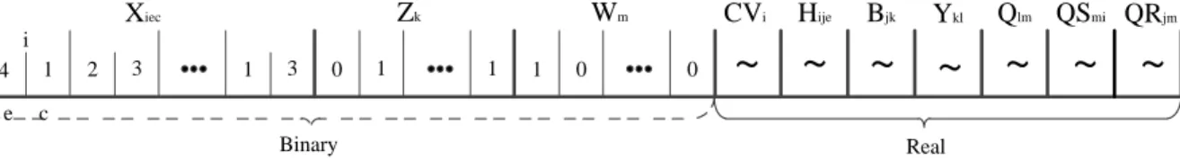
6-1-1- Chromosome representation
A vector like one depicted in Figure (2) is used to represent the chromosomes in proposed algorithm. In figure (2), solution string is divided into two parts: one for binary variables and another for real variables.
Binary variable part is coded by vectors 𝑧𝑧𝑘𝑘, wm, and 𝑥𝑥𝑖𝑖𝑐𝑐𝑐𝑐. A vector of ordered pairs is used to code 𝑥𝑥𝑖𝑖𝑐𝑐𝑐𝑐 which
determines the capacity and technology in initial product manufacturing plants. First element of this ordered pair
is assigned to technology and the latter is representative of capacity of plant 𝑀𝑀. The part related to real variables
is followed by binary variable part. This method of representing solutions results in feasibility of children solutions through crossover and mutations operators.
Xiec Zk Wm
i
e c
1
4 2 3 1 3 0 1 1 1 0 0
CVi Hije Bjk Ykl Qlm QSmi QRjm
~
~
~
~
~
~
~
Binary Real
Figure 2. Solution chromosome of proposed algorithm.
One of the difficulties of multi-objective optimization problems and Pareto frontier determination is to determine fitness of solutions and their survival transmission pattern to the next generation. Different methods
are proposed by previous studies to evaluate the solutions e.g. Deb et al. (2000) which is often based on the
quality of objective functions.
In proposed algorithm, objective functions are considered to evaluate fitness of solutions and their selection
is performed based on non-domination rank and crowding distance (Deb et al., 2000). In this approach, a
solution is non-dominated if it has less non-domination rank in the first instance, and if the solutions have the same non-domination rank solution with more crowding distance. So, the population is sorted and the best solutions are survived to the next generation.
It should be noted that in the proposed algorithm, to produce initial population and children through crossover and mutation, real variables of children are determined by solving linear programming model resulted from predetermined binary variables. In this linear programming model, random-weight method is applied to
change the problem to a single-objective one (Murata et al., 1996). This enables the algorithm to obtain a
uniform sample of Pareto solutions (Schaffer 1985). To reach this goal, objective functions are normalized and
rewritten as a weighted sum with random weights as presented in equation (56):
(56) 𝐶𝐶 = ∑3𝑖𝑖=1𝑤𝑤𝑖𝑖𝑓𝑓𝑖𝑖𝑛𝑛𝑛𝑛𝑛𝑛𝑚𝑚𝑎𝑎𝑙𝑙(𝑥𝑥)
where 𝑓𝑓𝑖𝑖𝑛𝑛𝑛𝑛𝑛𝑛𝑚𝑚𝑎𝑎𝑙𝑙(𝑥𝑥) is the th normalized objective function and 𝑤𝑤𝑖𝑖 is random weight related to that objective
function which should satisfy equation (57).
6-1-3- Crossover
In the proposed algorithm, one of the single point crossover, double point crossover and uniform crossover are selected randomly as the crossover operator of binary part of solutions. Applying any of these operators results’ in two children which their real part is obtained after solving the linear programming model with different weights for twice. If the solutions are feasible, real variables part of them are determined and four children are generated. If one or more of children become infeasible, numbers of feasible generated children would be less than the determined number which decreases the dispersion of search and as a result the efficiency of algorithm goes down. To prevent this, for real-variable part of children which have the same binary-variable part, crossover operator is applied and new children are generated. To recombine their real-variable part
Blending operator is utilized which is a linear random combination of parents.
6.1.4 Mutation
In the proposed algorithm, mutation operator is applied for binary variables. First, one of the elements of binary part of parents solution is selected randomly and then, suitable flip operation is performed according to
the fact that it is in 𝑧𝑧𝑘𝑘, 𝑤𝑤𝑚𝑚 or 𝑥𝑥𝑖𝑖𝑐𝑐𝑐𝑐 variable domain. In other words, if it is in 𝑧𝑧𝑘𝑘 or 𝑤𝑤𝑚𝑚 variable domain, it is
enough to exchange the element with the opposite value. But if it is in 𝑥𝑥𝑖𝑖𝑐𝑐𝑐𝑐 variable domain, the selected
element should exchange with a new and different value of available set.
6.1.5 Selection
Parents’ selection for crossover and mutation is based on elitism in proposed algorithm. In this method, certain fraction of the best elements of population can be uniformly selected. This method is able to strengthen convergence strategies with respect to extension of solution space.
7- Case study and results
We have performed a case study in a steel industry. In this network, scrap parts are collected and along with purchased raw material purchased are utilized for manufacturing products in raw steel plants as a forward flow. Then raw steel is shipped to other plants and final products are manufactured which are then shipped to demand (57) ∑3𝑖𝑖=1𝑤𝑤𝑖𝑖 = 1
markets through distribution centers. The used products and scrap of manufacturing plants are entered to collection centers to be sending and recycling in initial product manufacturing plants.
Data needed to solve the model, has collected from different sources such as steel industries experts, earlier studies (Vahdani et al., 2013 and Strezov et al., 2013) and ECO-it software (relating environmental issues) which is provided in Table 1.
Table 1.The data of the case study
Parameter Value Parameter Value
𝑝𝑝𝑐𝑐𝑖𝑖2𝑐𝑐 𝑈𝑈𝑀𝑀𝑀𝑀𝑓𝑓𝑓𝑓𝑓𝑓𝑚𝑚 (90 − 120) 𝑓𝑓𝑙𝑙 𝑈𝑈𝑀𝑀𝑀𝑀𝑓𝑓𝑓𝑓𝑓𝑓𝑚𝑚 (.2 − .35)
𝑗𝑗𝑐𝑐𝑗𝑗 𝑈𝑈𝑀𝑀𝑀𝑀𝑓𝑓𝑓𝑓𝑓𝑓𝑚𝑚 (25 − 35) 𝑓𝑓𝑗𝑗 𝑈𝑈𝑀𝑀𝑀𝑀𝑓𝑓𝑓𝑓𝑓𝑓𝑚𝑚 (.85 − .97)
𝑘𝑘𝑐𝑐𝑘𝑘 𝑈𝑈𝑀𝑀𝑀𝑀𝑓𝑓𝑓𝑓𝑓𝑓𝑚𝑚 (2 − 5) 𝐹𝐹𝐹𝐹𝑖𝑖11 𝑈𝑈𝑀𝑀𝑀𝑀𝑓𝑓𝑓𝑓𝑓𝑓𝑚𝑚 (330000 − 960000)
𝑚𝑚𝑐𝑐𝑚𝑚 𝑈𝑈𝑀𝑀𝑀𝑀𝑓𝑓𝑓𝑓𝑓𝑓𝑚𝑚 (2 − 5) 𝐹𝐹𝐹𝐹𝑖𝑖12 𝑈𝑈𝑀𝑀𝑀𝑀𝑓𝑓𝑓𝑓𝑓𝑓𝑚𝑚 (300000 − 900000)
𝑀𝑀𝐹𝐹𝑖𝑖1𝑐𝑐 𝑈𝑈𝑀𝑀𝑀𝑀𝑓𝑓𝑓𝑓𝑓𝑓𝑚𝑚 (1500 − 3000) 𝐹𝐹𝐹𝐹𝑖𝑖21 𝛼𝛼 ∗ 𝐹𝐹𝐹𝐹𝑖𝑖11
𝑀𝑀𝐹𝐹𝑖𝑖2𝑐𝑐 𝜆𝜆𝑀𝑀𝐹𝐹𝑖𝑖1𝑐𝑐 𝐹𝐹𝐹𝐹𝑖𝑖22 𝛼𝛼 ∗ 𝐹𝐹𝐹𝐹𝑖𝑖12
𝜆𝜆 𝑈𝑈𝑀𝑀𝑀𝑀𝑓𝑓𝑓𝑓𝑓𝑓𝑚𝑚 (.4 − .6) 𝛼𝛼 𝑈𝑈𝑀𝑀𝑀𝑀𝑓𝑓𝑓𝑓𝑓𝑓𝑚𝑚 (.5 − .7)
𝑀𝑀𝐶𝐶𝑗𝑗 𝑈𝑈𝑀𝑀𝑀𝑀𝑓𝑓𝑓𝑓𝑓𝑓𝑚𝑚(1500 − 3000) 𝑔𝑔𝑘𝑘 𝑈𝑈𝑀𝑀𝑀𝑀𝑓𝑓𝑓𝑓𝑓𝑓𝑚𝑚 (5000 − 10000)
𝑀𝑀𝐶𝐶𝑘𝑘 𝑈𝑈𝑀𝑀𝑀𝑀𝑓𝑓𝑓𝑓𝑓𝑓𝑚𝑚 (800 − 1800) 𝑓𝑓𝑚𝑚 𝑈𝑈𝑀𝑀𝑀𝑀𝑓𝑓𝑓𝑓𝑓𝑓𝑚𝑚 (1000 − 5000)
𝑀𝑀𝐶𝐶𝑚𝑚 𝑈𝑈𝑀𝑀𝑀𝑀𝑓𝑓𝑓𝑓𝑓𝑓𝑚𝑚 (800 − 1800) 𝑝𝑝𝑐𝑐𝑖𝑖1𝑐𝑐 𝑈𝑈𝑀𝑀𝑀𝑀𝑓𝑓𝑓𝑓𝑓𝑓𝑚𝑚 (60 − 90)
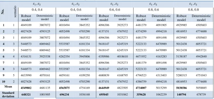
First, to show the efficiency of robust model in relation to deterministic model, third and fourth objective function are normalized and combined with the weights of 0.4 and 0.6. Then second and third objective
functions are considered as constraints and are solved with ɛ-constraint method for different values of . The
most probable scenario is taken into account as deterministic counterpart. To compare rest of the scenarios, the criterion is that if manufacturing quantity is less than quantity of the most likely scenario, shortage costs will be considered but if it is more than quantity of the most likely scenario, inventory costs will be included. Results of
10 randomly selected among 5 possible scenarios with different probabilities are gathered in Table 2 where 𝜀𝜀1
and 𝜀𝜀2 indicate second and third objective functions in normalized form respectively which are fixed to certain
amount and the amount of first objective function is reported. This table provides a comparison between deterministic and robust model in terms of average and standard deviation of the objective amounts of the 10 mentioned scenarios which indicates the efficiency of robust counterpart since mean and standard deviation of costs are less than deterministic model.
Table 2. Comparing robust and deterministic model
No . sce n ar io
𝜀𝜀1 , 𝜀𝜀2 𝜀𝜀1 , 𝜀𝜀2 𝜀𝜀1 , 𝜀𝜀2 𝜀𝜀1 , 𝜀𝜀2 𝜀𝜀1 , 𝜀𝜀2
0.4, 0.4 0.4, 0.6 0.6, 0.6 0.8, 0.6 0.8, 0.8
Robust model Deterministic model Robust model Deterministic model Robust model Deterministic model Robust model Deterministic model Robust model Deterministic model 1 1 4049109 3807072 4010494 3845352 4096306 3925273 4481379 4091905 4929985 4505603 2 2 4027428 4593125 4052498 4703290 4137151 4767932 4374299 4994218 4816953 4774688 3 1 4049109 3807072 4010494 3845352 4096306 3925273 4481379 4091498 4929985 4505603 4 3 5448573 6069462 5533587 6181334 5618147 6245319 5222133 6470989 5012438 6053721 5 3 5448573 6069462 5533587 6181334 5618147 6245319 5222133 6470989 5012438 6053721 6 4 4316131 3925338 4262354 3945806 4350986 4018610 4671952 4163283 5138187 4942840 7 1 4049109 3807072 4010494 3845352 4096306 3925273 4481379 4091498 4929985 4505603 8 3 5448573 6069462 5533587 6181334 5618147 6245319 5222133 6470989 5012438 6053721 9 5 4633990 4070161 4659161 4109250 4680839 4168795 4796523 4313403 5280315 4751043 10 2 4027428 4593125 4052498 4703290 4137151 4767932 4386759 4994218 4816953 4774688
Mean 4549802 4681135 4565875 4754169 4644949 4823505 4734007 5015299 5038586 5058885
Standard
The relationship between the total cost and infeasibility penalty of non-deterministic constraints is depicted in Figure 3. As can be seen, penalty cost increases exponentially as the total cost increases that is in accordance with what is addressed in Mulvey et al. (1995).
Figure3. Trade-off between 𝜔𝜔 and total cost
The proposed algorithm is programmed in MATLAB and its efficiency is checked by applying it on a
problem. In this regard, one of the objective functions is considered to be fix and the two others are compared
with solutions obtained from 𝜀𝜀-constraint approach which indicates little difference (Figure 4). It should be
noted that the objective functions are normalized and changed into maximization form in Figure 4.
Figure4. Comparing Results obtained from Genetic algorithms and GAMS
Resulted surface is depicted in Figures 5 and its two dimensional views are shown in Figure 6. Figure 5 and 6 show that increasing objective function of social utility results in an increase in cost objective function. We need to locate many small factories to increase fairness in distributing jobs in different spots and then to increase
social objective function. Also, we need more facilities and new technology to provide more job opportunities. As a result, costs increase and cost utility decreases. An increase in environmental objective function e.g. using green technology with less harm to environment causes increase in cost. Hence, decision maker decides about supply chain network by considering objective function’s utility.
Figure5. Pareto solutions surface for three objective functions problem
Figure6. Two dimensional view of Pareto surface
2 4
6 8
10 12
14 x 106
0 5000
10000 15000
0.2 0.4 0.6 0.8 1
Z
2
Z
1 Z 3
2 4 6 8 10 12 14
x 106 0
1 2x 10
4
1'th Objective
2'
th O
bj
ec
ti
v
e
2 4 6 8 10 12 14
x 106 0
0.5 1
1'th Objective
3'
th O
bj
ec
ti
v
e
0 2000 4000 6000 8000 10000 12000
0 0.5 1
2'th Objective
3'
th O
bj
ec
ti
v
8- Conclusion
In this paper a multi-objective model is proposed considering both forward and reverse flows of supply chain with objective functions designed for costs, environmental factors such as CO2 emission, and social factors such as employment and fairness in providing job opportunities according to ISO 26000 standards. A case study of steel manufacturing and recycling industry is presented since this industry is one of the important industries which creates vast job opportunities and has a great role in environmental contamination. Since demand has non-deterministic nature, a robust programming model is developed to cope with uncertainty and the mean and standard deviation of costs are taken into consideration. Results show that robust model is more efficient in relation to deterministic model. To solve the model, a multi-objective genetic algorithm is applied and results show its efficiency in generating Pareto solutions.
It seems that it is useful to consider multi-period and multi-product problems in future research. Considering different transportation modes and delineating appropriate ways of calculating economic, social and environmental impacts can be added to extend the study. For future direction, we suggest considering other environmental and social factors such as energy consumption level, local suppliers’ priority, industrial centers adjacency, and facilities’ distance related to providing new job opportunities.
References
Amin, S.H. & Zhang, G. (2013), A multi-objective facility location model for closed-loop supply chain network
under uncertain demand and return. Applied Mathematical Modeling, 37(6); 4165-4176.
Carter, C.R., Jennings, M.M. (2002), Social responsibility and supply chain relationships. Transportation
Research Part E: Logistics and Transportation Review, 38; 37-52.
Cruz, J.M. (2009), The impact of corporate social responsibility in supply chain management: Multicriteria
decision-making approach. Decision Support Systems, 48; 224-236.
Cruz, J.M. & Wakolbinger, T. (2008), Multiperiod effects of corporate social responsibility on supply chain
networks, transaction costs, emissions, and risk. International Journal of Production Economics, 116(1); 61-74.
Das, K. & Chowdhury, A.H. (2012), Designing a reverse logistics network for optimal collection, recovery and
quality-based product-mix planning. International Journal of Production Economics, 135(1); 209-221.
De Rosa, V., Gebhard, M., Hartmann, E. & Wollenweber, J. (2013), Robust sustainable bi-directional logistics
network design under uncertainty. International Journal of Production Economics, 145(1);184-198.
Deb, K., Pratap, A., Agarwal, S. & Meyarivan, T. (2002), A fast and elitist multiobjective genetic algorithm:
NSGA-II. Evolutionary Computation, IEEE Transactions on, 6(2); 182-197.
Deb, K., Agrawal, S., Pratap, A. & Meyarivan, T. (2000), A fast elitist non-dominated sorting genetic algorithm
for multi-objective optimization: NSGA-II. Lecture notes in computer science, 1917, 849-858.
Dehghanian, F. & Mansour, S. (2009), Designing sustainable recovery network of end-of-life products using
genetic algorithm. Resources, Conservation and Recycling, 53(10); 559-570.
Easwaran, G. & Üster, H. (2010), A closed-loop supply chain network design problem with integrated forward
and reverse channel decisions. IIE Transactions, 42(11); 779-792.
El-Sayed, M., Afia, N. & El-Kharbotly, A. (2010), A stochastic model for forward-reverse logistics network
Fleischmann, M., Beullens, P., Bloemhof-Rruwaard, J.M. & Wassenhove, L.N. (2001), The impact of product
recovery on logistics network design. Production and operations management, 10(2); 156-173.
Gen, M. & Cheng, R. (2000), Genetic algorithms and engineering optimization (Vol. 7): John Wiley & Sons.
Hasani, A., Zegordi, S.H. & Nikbakhsh, E. (2012), Robust closed-loop supply chain network design for
perishable goods in agile manufacturing under uncertainty. International Journal of Production Research,
50(16); 4649-4669.
Horn, J., N. Nafpliotis, and D.E. Goldberg. A niched Pareto genetic algorithm for multiobjective optimization.
in Evolutionary Computation, 1994. IEEE World Congress on Computational Intelligence., Proceedings of the
First IEEE Conference on. 1994: IEEE
ISO/TMB/WG/SR.(2006), Participating in the Future International Standard ISO 26000 on Social
Responsibility International Organization for Standardization, Geneva.
Keyvanshokooh, E., Fattahi, M., Seyed-Hosseini, S. & Tavakkoli-Moghaddam, R. (2013), A dynamic pricing
approach for returned products in integrated forward/reverse logistics network design. Applied Mathematical
Modeling, 37(24); 10182-10202.
Ko, H.J. & Evans, G.W. (2007), A genetic algorithm-based heuristic for the dynamic integrated forward/reverse
logistics network for 3PLs. Computers & Operations Research, 34(2); 346-366.
Lee, P.K.C. & Humphreys, P.K. (2007), The role of Guanxi in supply management practices. International
Journal of Production Economics, 106(2); 450-467.
Mulvey, J.M., Vanderbei, R.J. & Zenios, S.A. (1995), Robust optimization of large-scale systems. Operations
research, 43(2); 264-281.
Murata, T., Ishibuchi, H. & Tanaka, H. (1996), Multi-objective genetic algorithm and its applications to
flowshop scheduling. Computers & Industrial Engineering, 30(4); 957-968.
Özkır, V. & Başlıgıl, H. (2012), Modelling product-recovery processes in closed-loop supply-chain network
design. International Journal of Production Research, 50(8); 2218-2233.
Özkir, V. & Basligil, H. (2013), Multi-objective optimization of closed-loop supply chains in uncertain
environment. Journal of Cleaner Production, 41(0); 114-125.
Pishvaee, M.S., Rabbani, M. & Torabi, S.A. (2011), A robust optimization approach to closed-loop supply chain
network design under uncertainty. Applied Mathematical Modelling, 35(2); 637-649.
Pishvaee, M.S. & Razmi, J. (2012), Environmental supply chain network design using multi-objective fuzzy
mathematical programming. Applied Mathematical Modelling, 36(8); 3433-3446.
Pishvaee, M.S. & Torabi, S.A. (2010), A possibilistic programming approach for closed-loop supply chain
network design under uncertainty. Fuzzy Sets and Systems, 161(20); 2668-2683.
Pishvaee, M.S., Farahani, R.Z. & Dullaert, W. (2010), A memetic algorithm for bi-objective integrated
forward/reverse logistics network design. Computers & Operations Research, 37(6); 1100-1112.
Pishvaee, M.S., Jolai, F, & Razmi, J. (2009), A stochastic optimization model for integrated forward/reverse
Pishvaee, M.S., Razmi, J. & Torabi, S.A. (2012), Robust possibilistic programming for socially responsible
supply chain network design: A new approach. Fuzzy Sets and Systems, 206(0); 1-20.
Ramezani, M., Bashiri, M. & Tavakkoli-Moghaddam, R. (2013a), A new multi-objective stochastic model for a
forward/reverse logistic network design with responsiveness and quality level. Applied Mathematical Modeling,
37(1-2); 328-344.
Ramezani, M., Bashiri, M. & Tavakkoli-Moghaddam, R. (2013b), A robust design for a closed-loop supply
chain network under an uncertain environment. The International Journal of Advanced Manufacturing
Technology, 66(5-8); 825-843.
Salema, M.I.G., Póvoa, A.P.B. & Novais, A.Q. (2005), Design and planning of supply chains with reverse flows. Computer Aided Chemical Engineering, 20; 1075-1080.
Salema, M.I.G., Barbosa-Povoa, A.P. & Novais, A.Q. (2007). An optimization model for the design of a
capacitated multi-product reverse logistics network with uncertainty. European Journal of Operational
Research, 179(3): 1063-1077.
Schaffer, J.D. & Grefenstette, J.J. (1985), Multi-Objective Learning via Genetic Algorithms. In: IJCAI (Vol.
85, pp. 593-595): Citeseer.
Sim, E. Jung, H. Kim, & Park, J. (2004), A Generic Network Design for a Closed-Loop Supply Chain Using
Genetic Algorithm. Genetic and Evolutionary Computation - GECCO, 31; 1214-1225.
Srinivas, N. & Deb. K. (1994), Muiltiobjective optimization using nondominated sorting in genetic algorithms. Evolutionary computation,. 2(3); 221-248.
Strezov, V., Evans, A. & Evans, T. (2013), Defining sustainability indicators of iron and steel production.
Journal of cleaner production, 51; 66-70.
Subramanian, P., Ramkumar, N., Narendran, T.T. & Ganesh, K. (2013), PRISM: PRIority based SiMulated
annealing for a closed loop supply chain network design problem. Applied Soft Computing, 13(2); 1121-1135.
Vahdani, B., Tavakkoli-Moghaddam, R. & Jolai, F. (2013), Reliable design of a logistics network under
uncertainty: A fuzzy possibilistic-queuing model. Applied Mathematical Modeling, 37(5); 3254-3268.
Wang, H.-F. & Hsu, H.-W. (2010), A closed-loop logistic model with a spanning-tree based genetic algorithm.
Computers & Operations Research, 37(2); 376-389.
Wang, Y., Zhu, X., Lu, T. & Jeeva, A.S. (2013), Eco-efficient based logistics network design in hybrid
manufacturing/remanufacturing system in low-carbon economy. Journal of Industrial Engineering and
Management, 6(1); 200-214.
Yu, C.-S. & Li, H.-L. (2000), A robust optimization model for stochastic logistic problems. International
Journal of Production Economics, 64(1); 385-397.
Zitzler, E. & Thiele, L. (1999), Multiobjective evolutionary algorithms: a comparative case study and the
strength Pareto approach. Evolutionary Computation, IEEE Transactions on, 3(4); 257-271.
Zitzler, E., Laumanns, M. & Thiele, L. (2001), SPEA2: Improving the strength Pareto evolutionary algorithm. In: Eidgenössische Technische Hochschule Zürich (ETH), Institut für Technische Informatik und Kommunikationsnetze (TIK).