Recursive Tree Algorithms for Orthogonal Matrix
Generation and Matrix-Vector Multiplications in
Rigid Body Simulations
Fuhui Fang
∗April 5, 2016
Abstract
In this paper, we study a numerical linear algebra problem arising from the efficient simulation of Brownian dynamics with hydrodynamics interactions where molecules are modeled as ensembles of rigid bodies. Given the first 6 rows of a matrix Q of size 3n×3n describing how the force on each of the
n particles in a rigid body P can be mapped to the 6 entries in P’s resultant force and torque, we show how the remaining 3n−6 rows of vectors can be constructed explicitly using O(nlog(n)) operations and storage, so that (1) they form an orthonormal basis and (2) they are orthogonal to each of the first 6 vectors. For applications where only the matrix-vector multiplications are needed, without forming Q, we introduce O(n) recursive tree algorithms for computing both Q·~v and QT ·~v for an arbitrary vector ~v. Preliminary numerical results are presented to demonstrate the performance and accuracy of the numerical algorithms.
1
Problem Statement
Assume a rigid body P consists of n unit-mass particles Pj, j = 1,· · · , n and P’s
mass center is located at the origin O~ = (0,0,0)T. Further assume an external force
~
fj = (fj1, fj2, fj3)T is applied on particle Pj located at ~rj = (xj, yj, zj)T, then the
∗This project was supported by the Michael P. and Jean W. Carter Research Fund administered
resultant force f~P and torque~τP of rigid body P are given by
~ fP =
n
X
j=1
~
fj, ~τP = n
X
j=1
~
rj ×f~j, (1.1)
and the corresponding matrix form is given by
~
fP
~ τP
6×1
=
I I . . . I A1 A2 . . . An
6×3n
~ f1 ~ f2 · · · ~ fn
3n×1
=Z ~ f1 ~ f2 · · · ~ fn , (1.2)
where the 6×3n matrix Z is defined as
Z =
~ z1T
· · · ~ zT 6 =
I I . . . I A1 A2 . . . An
(1.3)
which will be referred to as the Z-matrix of P,I is the 3×3 Identity matrix, and Ai
represents the translation matrix of Ai ·f~i ,ri ×f~i which can be explicitly written
as
Ai =
0 −zi yi
zi 0 −xi
−yi xi 0
.
Note that when the Gram-Schmidt process is applied on the 6 row-vectors of Z, an orthonormal basis {~q1, ~q2,· · · , ~qk} can be derived using an upper triangular matrixR
of size 6×k as in
QZ ,[~q1, ~q2,· · ·~qk]T = (RT)−1·Z.
In this paper, we introduce three recursive tree algorithms to address the following three questions:
Q1: Given the 6 × 3n Z-matrix Z (or equivalently QZ = [q~1, ~q2,· · ·~qk]T) of a
rigid body P consisting of n particles, how to efficiently construct the remain-ing 3n − k orthonormal vectors ˜Q = [~qk+1, ~qk+2,· · · , ~q3n]T, such that the matrix
Q3n×3n =
QZ
˜
Q
is an orthogonal matrix?
Q2: For any given set of forces applied on thenparticles, how toefficientlycompute the matrix-vector multiplication
Q3n×3n
~ f1 · · · ~ fn
3n×1
? (1.4)
2
Background
The three questions arise in our research efforts to design optimal numerical tools for simulating the Brownian dynamics of biomolecules with hydrodynamics interac-tions, where a complex molecular system is modeled by multiple (e.g., hundreds or thousands) rigid bodies to reduce the numerical “stiffness” due to the local chemi-cal bond type interactions between atoms that cause very high frequency oscillations (which require extremely small time step sizes when marching in time). Instead of a thorough listing of existing literature on the Brownian dynamics models and hy-drodynamics interactions, we focus on the “bead model” in [9] in which a molecular system is modeled bymrigid bodies with given external forces{f~j}and torques{~τj},
j = 1,· · · , m, in each step of the dynamics simulation. To simplify the discussions and notations, we further assume that theZ-matrixof each rigid body has full rank 6 (lower rank cases can be handled similarly, but notations will be more involved). Un-der this assumption, the unknowns are then the size 3 translational velocity vectors
{~vj}and angular velocity vectors{~ωj},j = 1,· · · , m, which determine how each rigid
body moves. There are therefore a total of 6m unknowns, the same as the number of entries in the given forces and torques.
To simulate the hydrodynamics interactions of the molecular system, each rigid body is further modeled by a number of “beads” (usually of the same radius) placed on its surface. This can be roughly considered as a particle-type method for solving the boundary value Stokes equations. When nj beads are used for rigid body j,
the total number of beads is then n = Pm
j=1nj. The bead model assumes that
the hydrodynamics interactions satisfy D ~f = ~v, where D3n×3n is the
Rotne-Prager-Yamakawa tensor whose entries are determined by the bead locations (see, e.g., [1, 2]), f~ is a vector of size 3n consisting of n force vectors, each of which is of size 3 representing the force on each bead, and ~v is a vector of size 3n consisting of the three velocity components of each bead. Adding the rigid body constraints, the bead model can then be described by
Z6m×3nD−3n1×3nZ T
3n×6m
~v1
~ ω1
.. .
~vm
~ ωm
6m×1
=
~
f1
~τ1
.. . ~
fm
~ τm
6m×1
(2.1)
In the formula, Z6m×3n is a block diagonal matrix and each diagonal block is the
6×3nj Z-matrix of rigid bodyj in Eq. (1.3).
~
v1T, ~ω1T,· · · , ~vmT, ~ωTmT of the rigid bodies, ~vbead , Z3Tn×6m~vr body gives the velocity
vector of all the beads, f~bead , D3−n1×3n~vbead is then the force-and-torque vector of
all the beads due to the hydrodynamics interactions modeled by the Rotne-Prager-Yamakawa tensor. When the resultant force and torque vector of the rigid bodies is derived using the mapping f~r body , Z6m×3nf~bead, it has to match the given external
force and torque vector as in f~r body = f~ext ,
h
~
f1T, ~τ1T,· · · , ~fmT, ~τmT
iT
. We want to mention that instead of using the Z-matrix for each rigid body in Eq. (2.1), one can also consider the diagonalized formulation
QZ6m×3nD
−1
3n×3nQZT3n×6m˜v6m×1 = ˜f6m×1, (2.2)
where each diagonal blockQZj inQZcontains the orthonormal basis vectors ofZj, and
˜
v and ˜f are the corresponding vectors after performing the same orthogonalization procedure on the original f~ext and ~vr body vectors. One numerical difficulty when
solving Eq. (2.1) or Eq. (2.2) is the calculation of D−1: as D is a dense matrix, for large n, even with the acceleration of the fast direct solvers [3, 6] or H-matrix based techniques [4, 5], computingD−1 is simply too expensive in the dynamics simulations
as the solution of the bead model is required at each and every time marching step. To overcome this hurdle, in the following, we show how to reformulate Eq. (2.2) to a different linear system. The technique for Eq. (2.1) is very similar and we neglect the details in this paper. The first step is to form the orthogonal matrix QT
Z Q˜T
3n×3n,
and add 3n−6m zeros to ˜v6m×1, to form
QZ6m×3nD
−1 3n×3n
QTZ Q˜T 3n×3n
˜
v ~0
3n×1
= ˜f6m×1.
Next, we add 3n−6m new equations to the original system to form
QZ
˜
Q
3n×3n
D−3n1×3n QT Z Q˜T
3n×3n
˜
v
0
3n×1
= ˜
f ~g
3n×1
, (2.3)
where the vector ~g(3n−6m)×1 contains 3n−6m unknown numbers. We multiply both
sides by QT Z Q˜T
to get
D−1
QT Z Q˜T
˜ v 0 = QT Z Q˜T
˜
f ~g
=hQTZf˜+ ˜QT~gi, (2.4)
where we used the fact that QTZ Q˜T is an orthogonal matrix and its inverse is simply its transpose. Then, we multiply both sides of the equation by D to get
QTZ Q˜T
˜
v ~0
Finally we multiply the equation by
QT Z Q˜T
T
to get
˜
v ~0
=
QZ
˜
Q
D
h
QTZf˜+ ˜QT~g
i =
QDQT
Zf˜+ ˜QT~g
˜
QDQTZf˜+ ˜QT~g
. (2.5)
In the new formulation, for the given vector ˜f6m×1, one first finds the unknown vector
~g by solving
~0 = ˜QDQT
Zf˜+ ˜QDQ˜T~g (2.6)
using a preconditioned Krylov subspace iterative method, and then computes the velocity vector ˜v6m×1 by evaluating
˜
v =QZD(QTf˜+ ˜QT~g). (2.7)
Note that the fundamental building blocks required when applying a Krylov sub-space method for the new formulation are the fast matrix-vector multiplication al-gorithms for computing (a) D·~v, (b)
QTZ Q˜T ·~v, and (c)
QTZ Q˜T T ·~v for any given vector ~v. For (a), one of the authors and collaborators has developed fast
O(n) algorithms using the fast multipole method (FMM) [7, 8]. In this paper, we introduce O(n) recursive tree algorithms for (b) and (c). We want to mention that other reformulations for Eq. (2.2) or Eq. (2.1) are also possible, including techniques based on the Schur complement. These alternatives are also being studied and com-pared with the approach in this paper. Another closely related research topic is the design of effective preconditioners for Eq. (2.6). Results along these directions will be discussed in future papers.
3
Divide-and-Conquer and Recursive Tree
Algo-rithms
data are approximately uniformly distributed, the adaptive tree usually hasO(log(n)) levels, making it efficient to process and transmit any data on the tree structure with better numerical stability features. In this section, we discuss how to use the divide-and-conquer technique on the tree structures to design optimal algorithms for the 3 questions in Sec. 1.
3.1
Adaptive Tree Structure
We first discuss how to generate a spatial adaptive tree when simulating a molecular system modeled by multiple rigid bodies in the bead model. We assume each rigid body is “discretized” into a number of beads as discussed in Sec. 2 to capture the hydrodynamics interactions between rigid bodies. A hierarchical partition is then performed to divide the beads domain into nested cubical boxes, where the root box is the smallest bounding box that contains all the beads. Without loss of generality, the root box is normalized to size 1 in each side. The root box is partitioned along each dimension in the middle, resulting in 8 child boxes in 3 dimensions. A child box becomes a leaf node in the tree structure if it contains no more than s beads. To simplify the discussions, we set s = 1 in this paper. In our implementation, other s
values are also allowed after changing how leaf nodes are processed in the code. If a child box contains more thansbeads, it will be further partitioned and this procedure continues recursively. If a child box is empty (with no beads inside), it will be pruned off from the tree.
This hierarchical spatial partition procedure results in an adaptive tree structure withLlevels. At levell = 0, the root node is the bounding box of size 1, and we refer to the non-empty boxes of size 1/2l as the nodes at level l of the recursive partition
procedure. Each parent node is connected to each of its children and this parent-child relation can be represented by an “edge” in the tree structure. Note that each node may contain either≤sbeads, or a rigid body consisting of> sbeads. Also, when the beads are approximately uniformly distributed, the number of levels is asymptotically
L=O(log(n)), and the number of nodes isO(n). These estimates are not correct for very special bead distributions which are unlikely to happen in real applications.
3.2
Q1: Explicit Orthogonal Matrix Generation
Without loss of generality, we consider a single (instead of m) rigid body consisting of n beads and discuss Q1: Given the rank = 6 and size = 6×3n Z-matrix Z (or
QZ = [~q1, ~q2,· · ·~q6]
T
), how to efficientlyconstruct the remaining3n−6 orthonormal vectors Q˜ = [~q7, ~q8,· · · , ~q3n]
T
, such that Q=hQTZ,Q˜Ti
T
form an orthogonal matrix?
Note that there are multiple choices of ˜Q. For efficiency and stability considera-tions, we study how to utilize the divide-and-conquer strategy on the adaptive tree and generate a special structured ˜Q. We start from a 2-level setting where the parent rigid bodyP at level 0 is partitioned into two child nodes at level 1, child X withnX
beads and child Y containingnY beads (nX +nY =n), and
ZX =
I I . . . I A1 A2 . . . AnX
6×3nX
, and ZY =
I I . . . I B1 B2 . . . BnY
6×3nY
are the Z-matrices of X and Y, respectively. We assume both ZX and ZY have full
rank (=6) to simplify the discussion and notation, and the orthogonal sub-matrices ˜
QX (size (3nX −6)×3nX) and ˜QY (size (3nY −6)×3nY) satisfying ˜QX ⊥ ZX and
˜
QY ⊥ZY are already constructed for childX andY, respectively. The key question in
a divide-and-conquer algorithm then becomes“how to find parent P’s Q˜ matrix (size (3n−6)×3n) such that Q˜ ⊥ZP, where ZP = [ZX, ZY] is P’s Z-matrix ”?
One way to answer the question is to study the matrix
H =
ZX ZY
06×3nX ZY
˜
QX 0(3nX−6)×3nY
0(3nY−6)×3nX Q˜Y
3n×3n
. (3.1)
It is straightforward to verify that the matrix is full rank, and the vectors in the lower 3n−12 rows
˜
QX 0(3nX−6)×3nY
0(3nY−6)×3nX Q˜Y
(3n−12)×3n
of H are normalized, orthogonal to each other, and orthogonal to the vectors in the first 12 rows of H. This means that parent P’s ˜Q can readily “receive” the lower 3n−12 rows of vectors from its two children. For the remaining 6 row vectors in ˜Q
(referred to as the Residue Vectors in the remainder of this paper), a Gram-Schmidt procedure on the first 12 row vectors can be performed and the last 6 orthonormal vectors will be orthogonal to the vectors in Z and the 3n − 12 vectors from the children. The Gram-Schmidt procedure requires approximately O(n) operations and
We want to mention that when eitherZX orZY is not full rank (=6), for example,
when each child only contains 1 bead (referred to as the bead-bead case), we have
k =rank(Z) = 5 and rank(ZX) =rank(ZY) = 3, and the dimension of the Residue Vectors is then 3 + 3 −5 = 1; when child X has only one bead (rank(ZX) = 3)
and child Y contains a rigid body with l = rank(ZY) being either l = 5 or l = 6,
assuming the parent’sZ-matrixhas rankk (k = 5 ork= 6), then theResidue Vectors
has dimensionl+ 3−k. The computations in these special cases are briefly discussed next.
Bead+Bead: When a parent has two child nodes, each contains only one bead, then the rank of theZ-matrix of each node is 3, the parent’sZ-matrixhas rank 5, and the dimension of the Residue Vectors is 3 + 3−5 = 1. The vector can be explicitly computed by normalizing the vector
x1−x2
z2−z1
,y1−y2, z2 −z1
,−1,−(x1−x2) z2−z1
,−(y1−y2) z2−z1
,1
,
where the vectors (xi, yi, zi) (i= 1,2) are the bead locations.
Bead+Rigid Body: Consider a parent node with two children. Child X has more than 1 bead and child Y contains only a single bead. When computing parent’s
Residue Vectors , instead of the 12×3n matrix
ZX ZY
0 ZY
, one can also applying
the Gram-Schmidt procedure on the 9×3n matrix
ZX ZY
0 I
, where I is the 3×3 Identity matrix.
In the pseudo-code presented in Algorithm 1, we describe a recursive implemen-tation of the divide-and-conquer technique using the function Q gen to explicitly generate the orthogonal matrix Q by an upward pass in the tree structure. To esti-mate the algorithm complexity and storage requirement, we consider a system with
n beads and a tree withO(log(n)) levels. To generate the Residue Vectors for all the nodes in one level, by taking advantage of the sparse structures (many zeros in the vector which are unnecessary to calculate or store), approximately O(n) operations (to compute all the required inner products and correspondingResidue Vectorsfor all nodes in this level) and O(n) storage are required. As there are O(log(n)) levels, the algorithm therefore hasO(nlog(n)) complexity andO(nlog(n)) memory requirement.
3.3
Upward pass: Algorithm for Computing
Q
·
~
v
in Q2
In the Brownian dynamics application in Sec. 2, instead of explicitly generating Qand QT, one only needs the final matrix-vector multiplication results. In this
Algorithm 1Upward Pass to Explicitly Generate Q
1: function Q gen(node P)
2: if nodeP is childlessthen
3: formP’sZ-matrix ZP.
4: else
5: find child nodesX and Y of node P.
6: Q gen(node X)
7: Q gen(node Y)
8: formP’sZ-matrix using child nodes’Z-matrices ZX and ZY.
9: perform Gram-Schmidt procedure on first 12 rows of H.
10: if nodeP is root node then
11: output all 12 orthogonal vectors.
12: else
13: output the last 6 (or less) Residue Vectors .
complexity and storage to the asymptotically optimal O(n) when explicit Q is not required. We first introduce the following definitions and theorems.
Definition 1 For a node P containing n beads in the tree structure, its Info-set is defined as the size 6 vector
MP =
I I . . . I A1 A2 . . . An
~ f1 .. . ~ fn =Z
~ f1 .. . ~ fn
, (3.2)
where f~j =
fj1, fj2, fj3T is the force acting on bead j and Z is the node’s Z-matrix .
Similar to the multipole expansions in the fast multipole method (FMM), the size 6
Info-set from child nodes can be combined to form parent’sInfo-set , as described by the following theorem.
Theorem 2 Assume a parent node P contains 2child nodes, Child X withnX beads and Child Y with nY beads, respectively. Also assume X and Y’s Info-set are given by
MX =
I · · · I A1 · · · AnX
~ f1 .. . ~ fnX =ZX
~ f1 .. . ~ fnX ,
MY =
I · · · I B1 · · · BnY
˜ f1 .. . ˜ fnY =ZY
Then the parent P’s Info-set defined as
MP =
ZX ZY
~ fX ˜ fY =
I · · · I I · · · I A1 · · · AnX B1 · · · BnY
~ f1 .. . ˜ fnY (3.3)
can be computed from its two children as
MP =MX +MY. (3.4)
Definition 3 For a nodeP containingnbeads in the tree structure, its Inertia Matrix
NP is defined as the 6×6 matrix
NP =
I . . . I A1 . . . An
I AT
1
.. . ...
I AT n
=ZP ·Z
T
P. (3.5)
We have the following theorem for constructing the Inertia Matrix .
Theorem 4 Assume a parent node P contains 2child nodes, Child X withnX beads and Child Y with nY beads, respectively. Also assume child X’s Inertia Matrix is
NX =
I . . . I A1 . . . AnX
I AT
1
.. . ...
I AT nX
=ZX ·Z
T X,
and Child B’s Inertia Matrix is
NY =
I . . . I B1 . . . BnY
I B1T
.. . ...
I BT nY
=ZY ·Z
T Y.
Then parent P’s Inertia Matrix defined as
NP =
I . . . I I . . . I A1 . . . AnX B1 . . . BnY
I AT1
.. . ...
I ATnX I BT
1
.. . ...
I BT nY
=ZP ·ZPT (3.6)
can be computed by
The Inertia Matrix contains all the necessary information for generating the
Residue Vectorsfrom theZ-matrix. As discussed in previous subsection, for a parent nodeP, its ˜Qconsists of two parts: the 3n−12 orthonormal vectors from child nodes
X and Y, and the Residue Vectorsderived from the Gram-Schmidt procedure on the 12 row vectors in H as in
H1:12=
I . . . I I . . . I A1 . . . AnX B1 . . . BnY
I . . . I
0
B1 . . . BnY
12×3n
=
ZX ZY
0 ZY
=
RT
11 0
RT21 RT22
12×(k+l)
QZ
˜
Q0
(k+l)×3n
=RT ·Q,
(3.7)
whereZX and ZY are theZ-matrices of child nodesX andY, respectively, the upper
triangular matrix R is partitioned into four blocks, R11 is of size 6×k where k is
the dimension of P’s Z-matrix , R22 is of size 6×l where l is the dimension of the
subspace formed by the Residue Vectors , Q is partitioned into two row blocks, QZ
corresponds to the first k orthogonal vectors such that row vectors in QZ span the
same subspace as row vectors in parent’s Z-matrix , and ˜Q0 contains the Residue
Vectors of dimension l. For most settings, k =l = 6, other possible values of k and l
include 3 and 5 as briefly discussed in previous subsection for special settings. In the Gram-Schmidt procedure, if we require the diagonal entries ofR11 andR22
to be positive, then Q and R will be uniquely determined. As it is unnecessary to explicitly generate the Residue Vectors , we define the Residue as a vector of size
l ≤6, denoted by~P, to store the product of the Residue Vectors with a given vector
~v as follows.
Definition 5 The Residue of a parent nodeP is defined as the product of its Residue Vectors and a given vector ~v3n×1 denoted as~P = ˜Q0 ·~v = ˜Q0·[~vXT, ~vTY]T, where ~vX and~vY are entries in~v corresponding to children X and Y, respectively.
Notice that for parent P,
ZX ZY
0 ZY
·~v =
MP
MY
=
RT11 0
RT
21 RT22
QZ·~v
˜
Q0·~v
, (3.8)
where MP =
ZX ZY
·~v and MY =ZY ·~vY are respectively parent P and Child
as
H1:12·H1:12T =
ZX ZY
0 ZY
·
ZX ZY
0 ZY
T =
NP NY
NY NY
=RTQ·QTR =RT ·R,
(3.9) whereNP and NY are the symmetric Inertia Matrixof parent P and childY,
respec-tively, and Q and R are the QR-decomposition of the first 12 rows of H as shown in Eq. (3.7). For the most common case when l=k = 6, as
RT11·QZ·~v =MP,
RT21·QZ ·~v+R22T ·Q˜0·~v =MY,
one can work out~P explicitly as
~P = ˜Q0·~v = (R22T )
−1(M
Y −RT21·QZ~v) = (RT22)
−1(M
Y −R21T ·(R
T
11)
−1·M
P). (3.10)
In the formula, one only needs R(computed from the Inertia Matrix N) and Info-set
M to get~P, the explicit form of the Residue Vectors is not required.
It is interesting to compare above definitions with those in the fast multipole meth-ods (FMM). Each node’sInfo-set Mcollects and compresses information from beads, and sends to its parent. This is very similar to the “multipole coefficients” in FMM. The Inertia Matrix N stores the necessary information for finding the translation operator (R matrix) for deriving the Residue ~ from M. Using a procedure similar to the FMM upward pass, the residues of all the nodes can be computed using the recursive functioncompute residuein Algorithm 2. The complexity and storage of the algorithm can be estimated by checking the operations and memory requirement for each node in the tree structure. Notice that the Info-set is a vector of size 6, the
Inertia Matrix is a matrix of size at most 6×6, and the size of the Residue is no more than 6. Also, as only the matrix-vector multiplication results are required and it is unnecessary to compute or store theResidue Vectors . The operation counts and storage for the algorithm is therefore proportional to the total number of nodes in the tree structure. For most bead distributions, as the number of nodes in the tree structure is proportional to the number of beads n, the algorithm complexity and storage are both O(n).
3.4
Downward Pass: Algorithm for Computing
Q
T~
v
in Q3
We address Q3: the efficient computation of the matrix-vector multiplicationQT~v inAlgorithm 2Upward Pass to Compute Q·~v
1: function compute residue(node P)
2: if nodeP is childlessthen
3: compute Info-set MP and Inertia Matrix NP.
4: else
5: find child nodesX and Y of node P.
6: compute residue(node X)
7: compute residue(node Y)
8: construct P’s Info-set MP and Inertia Matrix NP from children’s.
9: compute P’s Residue~using Eq. (3.10).
We start from an observation from rigid body dynamics. Given the translational velocity V~ and angular velocity ~ω of a rigid body P consisting of n beads, and assuming that the reference point is the origin O~, then the velocity of bead i in the rigid body can be computed by
~vi =V~ +~ω×~ri.
In matrix form, the bead velocities are given by
~v1
· · ·
~vn
3n×1
=
I AT
1
.. . ...
I ATn
3n×6
~
V ~ ω
6×1
=ZT · ~
V ~ ω
6×1
, (3.11)
where Z is theZ-matrix of P. Notice that only 6 numbers in V~ and ~ω are needed to construct all beads’ velocities, assuming the location of each bead is known. We there-fore introduce the definition of RV-set (rigid body velocity set), a vector containing the 6 numbers.
Definition 6 The RV-set of a rigid bodyP consisting ofn beads is defined as a vector of size 6given by L=
h
~ VT, ~ωT
iT
describing how the rigid body moves. The velocities of the beads in the rigid body are given in Eq. (3.11).
In Eq. (3.11), instead of the Z-matrix Z, one can also change the basis and use the corresponding QZ containing the orthonormal vectors {q1T, qT2, · · ·, qkT}, where
k =rank(Z). Then for any given vector~v of sizek, aRV-set vectorLof size 6 can be found (may not be unique) such that ZT ·L=QT
Z~v =
Pk
j=0qjT ·vj. This observation
provides a way to store the necessary information in the linear combination of the vectors {qT
used to store the compressed information. Next, we show how the stored information can be passed to the child nodes in an adaptive tree.
Theorem 7 Assume a parent rigid body P is partitioned to child X with Z-matrix
ZX and child Y with Z-matrix ZY, and parent P’s Z-matrix is ZP = [ZX, ZY]. Also assume that
ZT X 0
ZT Y ZYT
=
QT Z Q˜T0
R11 R21
0 R22
=
QT
ZR11, QTZR21+ ˜QT0R22
(3.12)
where R11 and R22 are upper triangular matrices computed using the Inertia Matrix
. Then for any vector ~v = [v1,· · · , vk]T of the same size as rank( ˜Q0), there exist
RV-set vectors L˜X and L˜Y for child X and Y, respectively, such that
˜
QT0~v =
ZT X ·L˜X
ZT Y ·L˜Y
, (3.13)
where
( ˜
LX =−R−111R21R−221~v,
˜
LY = (I−R−111R21)R−221~v,
(3.14)
i.e., without explicitly using Q˜0, Q˜T0~v can be compressed and stored in the RV-set of
child nodes.
Theorem 7 suggests a recursive algorithm on the tree structure to compress the matrix-vector multiplication results, store in each node’sRV-set, and send to its child nodes. At the root node, consider the QR decomposition of the Z-matrix ZrootT =
QT
rootRroot where Rroot is computed using the Inertia Matrix Nroot, and the linear
combination of vectors in QZroot with coupling coefficients ~vroot can be be stored as
the root node’s RV-set given by Lroot = R−root1 ~vroot. For any child node, the linear
combination of the orthogonal vectors from all parent nodes can be computed using its parent’sRV-set plus linear combination of its parent’sResidue Vectors with given coupling coefficients, and can be stored as child’s RV-set , as shown in the following theorem.
Theorem 8 Consider a parent rigid body P with child nodes X and Y in the tree structure and assume P’s RV-set LP satisfies QTP~v1 = ZPT ·LP where QP represents all the orthogonal vectors from P’s parents and grandparents and ~v1 is the coupling
coefficient vector. Further assume that
˜
QT0~v2 =
ZXT ·L˜X
ZYT ·L˜Y
where Q˜0 contains P’s Residue Vectors , ~v2 is the corresponding coupling coefficient
vector, and L˜X and L˜Y are computed using Eq. (3.14). Then for the two child nodes
X and Y, the linear combination of the orthogonal vectors from QP and Q˜0 can be
stored in child nodes’ RV-set LX and LY as in
h
QTP Q˜T0
i ·
~ v1
~ v2
=QTP~v1+ ˜QT0~v2 =ZPT·LP+
ZXT ·L˜X
ZYT ·L˜Y
=
ZXT ·LX
ZT Y ·LY
, (3.15)
where LX =LP + ˜LX, LY =LP + ˜LY.
This theorem shows how parent’s information can be combined with the information from Residue Vectors and sent to its children. The recursive algorithm implementa-tion is presented as a pseudo-code in Algorithm 3. In the algorithm, we assume the
R matrix for each node is already computed in the upward pass discussed in Sec. 3.3.
Algorithm 3Downward Pass to compute QT ·~v
1: function combine ortho vec(node P)
2: if nodeP is root nodethen
3: compute P’s RV-set using Lroot =R−root1 ~vroot.
4: else
5: compute P’s RV-set using Theorem 8. 6:
7: if nodeP is leaf nodethen
8: output the linear combination result for the leaf node.
9: else
10: find child nodesX and Y.
11: combine ortho vec(node X)
12: compine ortho vec(node Y)
4
Numerical Results
As a prototype, we implement the recursive algorithms with Matlab, and preliminary numerical results for the first two algorithms (explicit Qand implicitQmethods) are presented in this section. More numerical experiments will be conducted in future papers.
4.1
Performance Measurement
As in previous analysis, in a system with n beads, if we explicitly generate the orthogonal matrix Q and compute the matrix-vector multiplication Q · ~v
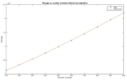
recursively, then the required storage is O(nlog(n)). With each choice of n
(n = 100,200,· · · ,1000), we run the algorithm ten times and obtain the average memory s used. Then we plot the required memory against the number of beads with a line of best fit using lease squares. As shown in Figure 1, the data points perfectly fit s = 32.1563nlog(n)−1628.7007, which corresponds to the O(nlog(n)) storage reqired.
Figure 1: Explicit QMethod, fitted line: s = 32.1563nlog(n)−1628.7007
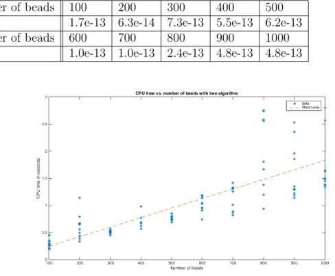
t= 0.0155nlog(n) + 53.6008 in Figure 2. This result verifies that the time complexity for the explicit Q method is O(nlog(n)). One problem with this figure is that the data points are located above the fitted curve when n = 100,200. Future work is required to improve the implementation.
Figure 2: Explicit Q Method, fitted line: t= 0.0155nlog(n) + 53.6008
Similarly, we run the second algorithm (the implicit Q method) ten times with the same choices of n, and we present the data points in Figure 3 with a fitted line
Table 1: Error Analysis: Q·QT −I
Number of beads 100 200 300 400 500
Error 1.7e-13 6.3e-14 7.3e-13 5.5e-13 6.2e-13
Number of beads 600 700 800 900 1000
Error 1.0e-13 1.0e-13 2.4e-13 4.8e-13 4.8e-13
Figure 3: Implicit Q Method, fitted line: t= 0.0011n+ 0.1763
4.2
Accuracy Measurement
We want to demonstrate that the Q generated explicitly is indeed orthogonal. In Table 1, we show that Q·QTI is close to machine precision, where I is the 3n×3n
identity matrix. Then we present the accuracy comparison from the two algorithms in Table 2 that shows that our algorithms guarantee the results are the same with a precision of at least 10 decimal digits. This number is less than machine precision, probably resulting from the QR-decomposition. If we create a matrixAbyA =Q·R, where Q is an orthogonal matrix and R is an upper triangular matrix, and then we perform QR-decomposition on A to form ˜Q and ˜R, then the norm of (Q−Q˜) and the norm of (R−R˜) may be zero with a precision of only 10 decimal digits. In other words, the Qwe generate explicitly and the Q used in the direct calculation of Q·~v
Table 2: Error Analysis: Explicit QMethod vs. Implicit Q Method
Number of beads 100 200 300 400 500
Error 5.5e-12 1.2e-11 2.8e-11 7.5e-11 9.5e-11
Number of beads 600 700 800 900 1000
Error 2.5e-10 4.7e-10 1.0e-10 9.5e-11 2.2e-10
Table 3: Error Analysis: QT ·Qv−v
Number of beads 100 200 300 400 500
Error 9.5e-13 2.4e-12 1.2e-11 4.2e-11 1.9e-11
Number of beads 600 700 800 900 1000
Error 1.4e-10 3.4e-11 3.2e-11 5.9e-11 2.4e-11
References
[1] GK Batchelor. Brownian diffusion of particles with hydrodynamic interaction.
Journal of Fluid Mechanics, 74(01):1–29, 1976.
[2] Donald L Ermak and JA McCammon. Brownian dynamics with hydrodynamic interactions. The Journal of chemical physics, 69(4):1352–1360, 1978.
[3] Leslie Greengard, Denis Gueyffier, Per-Gunnar Martinsson, and Vladimir Rokhlin. Fast direct solvers for integral equations in complex three-dimensional domains.
Acta Numerica, 18:243–275, 2009.
[4] Wolfgang Hackbusch. A sparse matrix arithmetic based on\ cal h-matrices. part i: Introduction to {\ Cal H}-matrices. Computing, 62(2):89–108, 1999.
[5] Wolfgang Hackbusch and Boris N Khoromskij. A sparse ?-matrix arithmetic.
Computing, 64(1):21–47, 2000.
[6] Kenneth L Ho and Leslie Greengard. A fast direct solver for structured linear systems by recursive skeletonization. SIAM Journal on Scientific Computing, 34(5):A2507–A2532, 2012.
[7] Shidong Jiang, Zhi Liang, and Jingfang Huang. A fast algorithm for brownian dy-namics simulation with hydrodynamic interactions. Mathematics of Computation, 82(283):1631–1645, 2013.