ORIGINAL ARTICLE
Detecting Chaotic Behavior in Agricultural Exchange-traded Funds
Jo-Hui Chen1, Tushigmaa Batsukh2,Yu-Fang Huang3
1Dept. of Finance, Chung Yuan Christian University, Chung Li, Taiwan, R.O.C. [email protected]
2Dept. of Business Administration, Chung Yuan Christian University, Chung Li, Taiwan, R.O.C. [email protected] 3Fu Jen Catholic University, Taipei, Taiwan, R.O.C. [email protected]
Abstract: This study investigates the chaos effect of agricultural exchange-traded funds (ETFs) using Brock, Dechert, and Scheinkman test, rescaled range analysis, and correlation dimension analysis. The standardized residuals from generalized autoregressive conditional heteroskedasticity models are fitted into eight ETFs and examined in each case for evidence of chaotic behavior. This study also examines whether or not the ETFs are consistent with the chaos effect based on the underlying random data with trend-reinforcing series. Research results outline the financial insights for the agricultural ETF field of investment forecasting to eliminate trading emotions, while pursuing considerable profitable experience for investors.
Keywords: agricultural ETF, chaos effect, brock dechert scheinkman test, rescaled range analysis, correlation dimension analysis
1. Introduction
In recent years, agricultural commodities have become popular choices because of the increasing number of people seeking anti-inflationary investments and because of land scarcity. Inamuraet al.[1]and Tang and Xiong[2]asserted that
in evaluating the extent of global commodity markets to examine the sensitivity of portfolio investment, commodity prices are significantly correlated with one another and greatly influence stock prices.
Exchange-traded funds (ETFs), which trace the advent of financial futures, are one of the most successful financial innovations introduced in the early 1990s as an investment fund traded on the U.S. and Canadian exchanges. Since its establishment in 2004 by ETF providers, a commodity ETF has become a useful tool for constructing diversification in investment portfolios and has been hedged against economic downturns (Ilanet al.[3]). A new investment opportunity of
agricultural ETFs is a topic that has recently received substantial attention from economists. Agricultural ETFs are one of the most effective means to diversify or stabilize a portfolio, hedge risk to invest in a broad agriculture fund, or focus on a specific commodity such as sugar, coffee, or grains. Using the returns of agricultural ETFs and futures relationship, Tse[4]posited that agricultural ETFs are significantly related to the stock market. Stock market sentiment is seen as a
key factor driving price behaviors.
The possible existence of nonlinear dynamic causes problems in forecasting financial and economic time series when linear models are applied. The literature has documented that chaotic series refer to the linear models (e.g., time series or regressions) that cannot capture regularities in such a series (Kohzadiet al.[5]). Chaotic systems based on
generally nonlinear response systems composed of erratic behavior, amplified events, and discontinuities. Benhabib and Nishimura[6], Grandmont[7], Day[8], Wolff[9], and Guegan and Leroux[10]have utilized the dynamical chaotic systems in Copyright © 2018 Jo-Hui Chenet al.
doi: 10.18686/fm.v3i1.866
This is an open-access article distributed under the terms of the Creative Commons Attribution Unported License
(http://creativecommons.org/licenses/by-nc/4.0/), which permits unrestricted use, distribution, and reproduction in any medium, provided the original work is properly cited.
economics and finance. These experts suggested that the character of noise is a distraction in a real data set by using chaos theory in practice, and that perceived development of robust deconvolution techniques is required. LeBaron[11]
argued that in financial markets, nonlinear forecasting may vary from actual chaotic dynamics.
In related studies, DeCosteret al.[12]applied correlation dimension to daily futures prices of sugar, silver, copper,
and coffee. Yang and Brorsen[13]employed correlation dimension and Brock, Dechert, and Scheinkman (BDS) test on
futures markets to examine the price changes for soybean, corn, and wheat. Bacsi[14] applied a linear cobweb model
along with Lyapunov models to analyze the weekly price of potatoes. Based on a deterministic price model unrelated to any stochastic component, the results observed irregular oscillations for fluctuations in real price series. Chatrath et al.[15]estimated the correlation dimension and BDS test on the daily prices of futures contracts for soybean, corn, cotton,
and wheat. The results revealed strong evidence of nonlinear dependence, which is not consistent with a long-lasting chaotic structure. Chappell and Panagiotidis[16]and Mahmoodzadehet al.[17]used the correlation dimension to examine
the nonlinear dynamics of the stock index and exchange rates of Athens. However, the findings contradicted the chaotic behavior and indicated the presence of low chaotic dimensions.
Substantial literature has explored chaotic behavior in food commodity. By contrast, no study has looked into whether agricultural ETFs exhibit chaotic dynamics. Therefore, this study aims to examine chaos structure in the daily price of agricultural ETFs by employing three different methods (i.e., BDS test, rescaled range (R/S) analysis, and correlation dimension analysis). The BDS test for nonlinearity detection and rescaled range (R/S) analysis confirm the existence of chaotic behavior in price. Correlation dimension verifies the results of R/S analysis. Through the analysis of chaotic effect for agricultural ETFs, investors can effectively use to predict tools to form investment decisions on agricultural futures and instruments.
The rest of this paper is organized into four sections. Following the Introduction, Section II explains the data as well as BDS test, R/S analysis, and correlation dimension analysis. Section III discusses the empirical results, and Section IV presents the conclusions of the study.
2. Data and Methodology
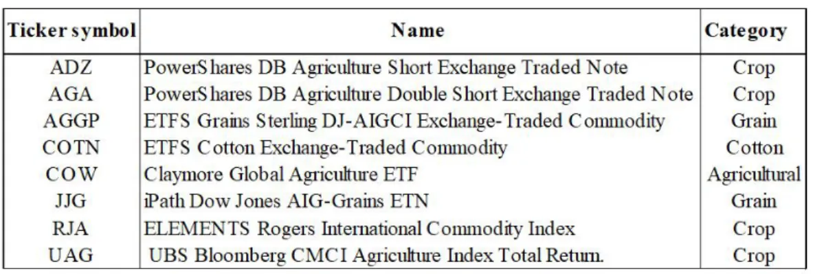
This research uses daily closing prices of eight agricultural ETFs (i.e., ADZ, AGA, UAG, RJA, JJG, AGGP, COTN, and COW) obtained from Yahoo! Finance. The agricultural ETFs data set is tabulated in Table 1. ADZ and AGA ETFs are issued by PowerShares Capital Management LLC. These indices are examined by tracing the performance of several agricultural futures contracts (e.g., corn, wheat, soybean, and sugar) and financial futures for the returns from investing in U.S. Treasury Bills for three months. The UAG issued by the Union Bank of Switzerland is adopted to measure the from futures contracts for collateralized returns representing the agricultural sector. RJA represents the value of a basket of 20 agricultural commodity futures contracts and is a subindex of the Rogers International Commodity Index issued by Merrill Lynch, Pierce, Fenner & Smith, a subsidiary of the Bank of America. JJG is composed of three futures contracts on grains traded on the U.S. exchange and used by Barclays iPath. All these preceding ETFs are listed on the New York Stock Exchange. AGGP and COTN are listed on the London Stock Exchange and are issued by ETF Securities, which tracks the Dow Jones-AIG (DJ-AIG) Grains Subindex and DJ-AIG Cotton Subindex and pay a capitalized interest return. COW is listed on the Canadian Toronto Stock Exchange and is issued by the Claymore Investments, Inc., which traces the performance of the MFC Global Agriculture Index.
Table 1. Data name and category
The data used in this study are those that fall between April 2008 and January 2011. As previously mentioned, this research applies three different approaches (i.e., BDS test, R/S analysis, and correlation dimension analysis) to explore chaotic behavior. Empirical research on finance and economics uses chaos theory to examine the nonlinear effects in deterministic systems transformed into a usable predictor of certain behavior (Djavanshir and Khorramshahgol[18]).
2.1. BDS statistics
The BDS test developed by Brocket al.[19][20]is superior to the alternative of deterministic chaos or stochastic nonlinear
models. The null hypothesis states that certain variables have the independently and identically distribution (i.i.d.) against the unspecified alternative. The calculations of BDS test begin with a given time series {xt} containing N observations, which should be the first difference of the natural logarithms of raw data in the time series to set up m-dimensional vectors called m-histories,
x
mt
x
t,
x
t1,...,
x
tm1
. These m-histories, collectively known as the embedding dimension, can be used to describe a correlation integral.
2
,
/
1
,
,
1 1 1
Tm mt m m
m u m t T
t
I
T
T
T
m
C
(1)where
T
m
T
m
1
, andI
x
tm,
x
sm
is an indicator function of the event
m t s i i
m s m
t
x
x
x
x
0max
.1.,.. 1 1 . (2)To calculate the pairs of the correlation integral lying within the tolerance distance ε for the embedding dimension m and the time series of length T, the BDS statistic is defined as
mT
T
mT
Tm
T
C
C
BDS
2 . 1. .1
.
/
. (3)2.2 R/S analysis
R/S analysis, which was invented by Hurst[21], is used mainly to estimate the repeated patterns in a time series of financial data. Given a time series, t, and all observed values, u, the estimation process is interpreted as follows:
t
1
u u N
N
t, (e M )
X , (4)
where ᴀ is the cumulative deviation over N periods, eu stand for the influx in year u, and MNrepresents the average
euover N periods. The range becomes the difference between maximum and minimum levels obtained from Equation
(4).
X
t,NMin
X
t,NMax
R
, 1 ≤ j ≤ n , (5)where R is the range of X, Max(X) is the maximum value of X, and Min(X) is the minimum value of X.
This range is divided by Hurst to measure the standard deviation, S, of the original observation to compare the different types of time series. The “rescaled range” should increase with time, and can be determined with the following formula:
R/S = (an)H, (6)
where R/S is the rescaled range, N is the number of observations, a is a constant, and H is the Hurst exponent.
Based on the series in a consistency of random walk, H is equal to 0.5. However, the observations are dependent when H is not 0.5. Each observation theoretically carries a long-term “memory” process of all the events that precede and last forever. Hurst statistic is interconnected through a long stream of events. To estimate the Hurst exponent, the natural logarithm is rewritten as below.
) ln( ) ( ) (
ln H an
n S n R
, H = ln (R / S) / ln (an). (7)
If H is 0.5, then the underlying time series has no correlation; 0 ≤ H<0.5. In this case, the time series increments
represent a related coefficient smaller than 0, and therefore, are negatively correlated with one another. If 0.5<H<1,
then the time series increments reveal a related coefficient which is larger than 0, indicating a positive correlation.
2.3 Correlation dimension analysis
The correlation dimension analysis was devised by Grassberger and Procaccia[22]. This technique measures the random
time series from the chaotic one. In this study, the correlation dimension algorithm is realized through four procedures explained below.
(1) Residual analysis is performed to remove autocorrelation and conditional heteroskedasticity.
(2) The information embedded dimension n estimates only the process of embedding the dimension value, which is not greater than the length of the original sequence, V, but is not less than 1. 1-history is expressed as
x
t1
x
t, 2-history is
t t
t
x
x
x
2 1,
, and n-history isx
tn
x
tn1,
...
,
x
t
, which signifies a point in n-dimensional space (n is the “embedding dimensions”).(3) The correlation integral is determined. Grassberger and Procaccia[22] used the integration process as
th t ᴀh ᴀa m ᴀhᴀ m a m . (8)
where # is the number of elements in the set, and the measurement of ( n u
x
,x
tn) distance implies that
.
(4) The minimum value of ε denotes the slope for the calculation of demand, and ‖‖ is calculated with the following formula:
log
/
log
lim
0 nn
C
v
. (10)When n increases, the correlation dimension
v
n increases continuously, revealing that the data do not have a fractal structure without a compliance characteristic of chaotic systems (Chappell and Panagiotidis[16]).3. Empirical Results
3.1 BDS test results
Price series and futures prices contain mostly unit roots, and are nonstationary (Moore and Cullen[23]; Beck[24]). Hence,
stationarity should be tested first before taking the nonlinearity test. In this study, the stationarity test is performed using the augmented Dickey–Fuller unit root test proposed by Dickey and Fuller[25]to examine the presence of unit root in the
series (difference stationarity). The agricultural ETF series is filtered with autoregressive integrated moving average (ARIMA) model and autoregressive conditional heteroskedasticity (ARCH) models to delete linear dependence and to eliminate the conditional heteroskedasticity, respectively. The generalized autoregressive conditional heteroskedasticity (GARCH) model is also used to reduce conditional heteroskedasticity. The standardized residuals of GARCH are likewise employed.
After the ETF series is filtered with GARCH model, BDS test statistics are estimated for ARIMA and GARCH filtered residuals as well as for the series compared before filtering. The null hypothesis of the BDS test based on underlying data following i.i.d is rejected. This condition suggests that the data are not i.i.d. because a nonlinear dependence is observed in the time series after the first differences of the natural logarithm are obtained. Table 2 compiles the BDS test results and shows that the JJG series is insignificant when the m embedding dimension is equal to 2. When the σ standard deviation ranges from 1 to 2, the BDS statistic results are insignificant. The results of the ARIMA filtered residuals indicate that AGGP, COW, ADZ, and COTN all have 1% significance level. The estimation of GARCH filtered residuals shows that the results of JJG, GOTN, and RJA are insignificant, whereas those of AGGP series are significant. However, the remaining four series are determined to be insignificant when σ standard deviation increases to 1, 1.5, and 2.
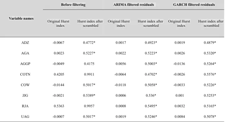
3.2 R/S analysis results
An H value of 0.5 designates a random series. An H value of more than 0.5 indicates a trend-reinforcing series, whereas large H values signify strong trends. Table 3 shows that the original values of H are mostly lower than 0.5. After the data are disordered, all values of H are determined to be significantly asymptotic to 0.5. The results reveal that the underlying data have a persistent and trend-reinforcing series. This finding illustrates that the upward or downward trend of the selected agricultural ETFs in the past would continue to be either positive or negative in the subsequent periods.
3.3 Correlation dimension analysis results
located on the horizontal and vertical axes, respectively. The eight-series correlation dimension evidently becomes convergent when the embedding dimension is at least greater than 4. This condition implies that the primary data of the agricultural ETFs may be chaotic.
Table 3 Empirical result of rescales range analysis test
Variable names
Before filtering ARIMA filtered residuals GARCH filtered residuals
Original Hurst
index Hurst index afterscrambled Original Hurstindex Hurst index afterscrambled Original Hurstindex Hurst index afterscrambled
ADZ -0.0067 0.4772* 0.0017 0.4923* 0.0019 0.4879*
AGA 0.0023 0.5227* 0.0022 0.5223* 0.0026 0.5320*
AGGP -0.0049 0.4175 0.0056 0.5003* -0.0136 0.5264*
COTN 0.4205 0.9911 -0.0064 0.4702* -0.0026 0.5576*
COW -0.0144 0.5017* -0.0118 0.5058* -0.0033 0.5226*
JJG -0.0021 0.5389* 0.0006 0.536* 0.001 0.5253*
RJA 0.5363 0.9957 0.0008 0.5495* 0.0032 0.5165*
UAG -0.0007 0.5017* 0.0019 0.5246* 0.0084 0.5078*
Note:*denotesH= 0.5;**denotes 0 ≤ H<0.5;***denotes 0.5<H<1.
4. Conclusion
This study applies BDS test, R/S analysis, and correlation dimension analysis, as well as with ARIMA and GARCH residual tests to examine the chaotic behavior of eight agricultural ETFs. The BDS results demonstrate that all agricultural ETFs are significant for the data before being filtered by ARIMA and GARCH models. The ARIMA residuals are also identified to be significant. If the series of the GARCH filtered residuals is verified to be non i.i.d., then the presence of nonlinear dependence may be observed. However, deterministic chaos could probably exist if the null hypothesis is not accepted. The GARCH filtered results are merely significant for the series of AGGP ETF. The BDS results contradict the expectation of this study, but are consistent with previous research that BDS may not be strong enough to examine weak nonlinearity (Wanget al.[26]). For R/S analysis, the underlying data are determined to
have a random and trend-reinforcing series. This observation specifies that the returns of agricultural ETFs are fractal and chaotic. The correlation dimension values are calculated against the corresponding embedding dimension, and all time series converge as expected. This finding demonstrates that the underlying data of agricultural ETFs are consistent with chaos and that conventional linear models are not appropriate for use in analyzing such ETFs.
In sum, this study verifies that a nonlinear and possibly chaotic structure may exist in the price series of all analyzed agricultural ETFs. Among all methods applied in this study, the R/S analysis provides the strongest results and verifies the uncertainty in the overall empirical results. Therefore, the findings presented in this paper can be adopted by future researchers or investors to forecast or form investment decisions.
References
1. Inamura Y, Kimata T, Kimura T, Mutto T, 2011, Recent Surge in International Commodity Prices-impact of Financialization of Commodities and Globally Accommodative Monetary Conditions. Bank of Japan Review, 2011-E-2.
2. Tang K and Xiong W, Index Investment and Financialization of Commodities. Princeton University and NBER Working Paper. 2010.
3. Ilan G, Li G, MaCann C, Futures-based Commodities ETFs. Securities Litigation and Consulting Group, Inc. 2011.
4. Tse Yiuman, The Relationship Among SAgricultural Futures, ETFs, and the US Stock Market. Review of Futures Markets, 2012, 20 (2): 141-159.
5. Kohzadi N, Boyd M S, Kermanshahi B, Kaastra I, A Comparison of Artificial Neural Network and Time Series Models for Forecasting Commodity Prices. Neurocomputing, 1996, 10: 169-181.
6. Benhabib J and Nishimura K, The Hopf Bifurcation and the Existence and Stability of Closed Orbits in Multi Sector Models of Optimal Economic Growth. Journal of Economic Theory, 1979, 21(3): 421-444.
7. Grandmont J M, Nonlinear Economic Dynamics. NY, Academic Press. 1988.
8. Day R H, Complex Economic Dynamics: Obvious in History, Generic in Theory, Elusive in Data. Journal of Applied Econometrics, 1992, 7: 9-23.
9. Wolff R C L, Local Lyapunov Exponents: Looking Closely at Chaos. Journal of the Royal Statistical Society, 1992, 54(2): 353-371.
10. Guegan D and Leroux J, Local Lyapunov Exponents: A New Way to Predict Chaotic [In Press]. Topics on Chaotic Systems, Systems World. 2007.
11. LeBaron B, Chaos and Nonlinear Forecastability in Economics and Finance. Philosophical Transactions of Royal Society of London Series a Physical Sciences and Engineering, 1994, 348(1688): 397-404.
12. DeCoster G P, Labys W C, Mitchell D W, Evidence of Chaos in Commodity Futures Prices. Journal of Futures Markets, 1992, 12(3): 291-305.
13. Yang S and Brorsen B W, Non-linear Dynamics of Daily Futures Prices: Conditional Heteroskedasticity or Chaos? Journal of Futures Markets, 1993, 13(2): 175-191.
14. Bacsi Z, Modelling Chaotic Behaviour in Agricultural Prices Using a Discrete Deterministic Nonlinear Price Model. Agricultural Systems, 1997, 55 (3): 445–459.
15. Chatrath A, Adrangi B, Dhanda K K, Are Commodity Prices Chaotic? Agricultural Economics, 2002, 27(2): 123-137.
Stock Exchange. Finance Letters, 2005, 3(4):29-32.
17. Mahmoodzadeh S, Shahrabi J, Pariazar M, Zaeri M S, Project Selection by Using Fuzzy AHP and TOPSIS Technique. World Academy of Science, Engineering and Technology, 2007, 30: 333-338.
18. Djavanshir G R and Khorramshahgol R, Applications of Chaos Theory for Mitigating Risks in Telecommunication Systems Planning in Global Competitive Market. Journal of Global Competitiveness, 2006, 14(1): 15-24.
19. Brock W A, Dechert W and Scheinkman J, A Test for Independence Based on the Correlation Dimension, Working paper, University of Winconsin at Madison, University of Houston, and University of Chicago. 1987.
20. Brock W A, Dechert W, Scheinkman J A, Lebaron B, A Test for Independence Based on the Correlation Dimension. Econometric Reviews, 1996, 15(3): 197-235.
21. Hurst H E, Long-term Storage Capacity of Reservoirs. Transactions of the American Society of Civil Engineers, 1951, 116: 770-799.
22. Grassberger P and Procaccia I, Measuring the Strangeness of Strange Attractors. Physical Review, 1983, 9:189-208.
23. Moore M J and Cullen U, Speculative Efficiency on the London Metal Exchange.The Manchester School, 1995, 63(3): 235-256.
24. Beck S, Autoregressive Conditional Heteroscedasticity in commodity spot prices. Journal of Applied Econometrics, 2001, 16(2): 115-132.
25. Dickey D A and Fuller W A, Distribution of the Estimators for Autoregressive Time Series with a Unit Root. Journal of the American Statistical Association, 1979, 74(366): 427–431.
26. Wang W, Vrijling J K, Pieter H A, Gelder V, Ma J, Testing for Nonlinearity of Streamflow Processes at Different Timescales. Journal of Hydrology, 2005, 322(1): 1-22.