Vol. 12, No. 1, pp 35-69
Concepts and Tests for Trend in Recurrent Event
Processes
R. J. Cook, J. F. Lawless
Department of Statistics and Actuarial Science, University of Waterloo, Ontario, Canada.
Abstract. Interest in the presence and nature of trend arises frequently
in science, public health, technology, and many other areas. In this ar-ticle we discuss the notion of trend in the context of recurrent event processes. We discuss different frameworks within which one can inves-tigate trend and consider various ways in which trends may be manifest. Tests for trend are discussed in detail and the utility of intensity-based models is emphasized for characterizing event processes and understand-ing trends. Simulation studies are conducted to study the effect of het-erogeneity in the investigation of trend. Data from a study of hospi-talization patterns in patients with affective disorder are analysed for illustration.
Keywords. Intensity function, recurrent events, robust methods,
stochas-tic modeling, trend.
MSC: 62N01, 62N02, 62N05, 62P10, 62P30, 62M05, 62M09.
1
Introduction
Processes of recurrent events are of interest in many settings, including medicine, sociology, economics and reliability (Cook and Lawless, 2007). In analysing such data, we are generally interested in understanding R.J.Cook( )([email protected]), J.F.Lawless([email protected])
Received: September 23, 2011; Accepted: June 29, 2012
aspects of the stochastic mechanism generating the events. This leads to consideration of models for the process intensity function, which specifies the probability of a new event at time t, given the previous history of event occurrences. In many situations the question arises about the presence and nature of trend. We discuss definitions of trend in what follows but, broadly speaking, the term refers to systematic variation in either event occurrence rates or times between events. Trends, as we discuss them, are monotonic (increasing or decreasing), which is in line with both the dictionary definition of trend as a general direction or tendency, and the common view of trend in time series (White and Granger, 2011).
Trends in recurrent event processes were discussed at some length by Cox and Lewis (1966), who gave a number of tests for trend in settings where there were no covariates. These and subsequent tests proposed in the literature assume a specific family of models within which certain sub-models are said to be trend-free. However, for models of recurrent events there is no universally adopted definition of a trend-free process or a process with trend (Ascher and Feingold, 1984, Section 9A). This is also true in other settings; in a review of trends in time series, White and Granger (2011) noted that “there is no generally accepted defini-tion” of trend. Despite this, when certain types of trends are present they are often readily apparent in plots. In medical research, studies typically involve multiple individuals with covariates, however, and in that case simple plots may not provide clear evidence concerning trend. For example, a tendency for times between hospitalizations for psychi-atric patients to decrease has been proposed (Kvist et al., 2008), but as we discuss later, this is difficult to establish.
The purpose of this paper is to review concepts of trend in recurrent event processes and the contexts in which they arise. We will focus on problems arising in chronic disease processes and on trends that manifest themselves at the individual subject level. Typical data sets involve many subjects but perhaps a rather small average number of events per subject. Standard notation and terminology for recurrent events will be used, as discussed by Cook and Lawless (2007).
Consider an individual process which starts at a designated time
t= 0, and letN(t) denote the number of events in (0, t]. The history of event occurrence at timet is denoted byH(t) and includes the number of events, N(t) = n, and their respective times 0 < T1 < · · · < Tn <
t. The times between events are called gap times and are denoted by
Wj =Tj −Tj−1 (j = 1, . . . , n), where T0 = 0. Unless stated otherwise
we consider processes in continuous time in which case the intensity function
λ(t|H(t)) = lim ∆t↓0
Pr{N(t+ ∆t)−N(t) = 1|H(t)}
∆t (1.1)
fully specifies the recurrent event process (Cook and Lawless, 2007, p. 10). Other features of a process that we consider are the marginal mean and rate functions, defined as
µ(t) =E{N(t)}, ρ(t) =dµ(t)/dt,
respectively.
As noted above, there is no universal definition of trend, or of its absence. The most common definitions of “no trend” are that either (a) the gap times Wj are identically distributed for j = 1,2, . . . or (b)
the rate function ρ(t) is a constantα. The special case of (a) in which the Wj are also assumed to be independent gives a renewal process.
Then, ρ(t) approaches the value α = E(Wj)−1 as t → ∞ although it
may vary substantially for small values of t. Another special process is the equilibrium renewal process; this is a “delayed” renewal process for which Wj (j = 2,3, . . .) are i.i.d. with distribution function F(w) and
survivor function S(w), but with W1 having density function f1(w) =
µ−1S(w), where µ = E(Wj), j = 1,2, . . . (Cook and Lawless, 2007,
p. 148). The equilibrium renewal process has constant rate function
ρ(t) = α = µ−1. Such processes are sometimes useful when the time
t = 0 indicates when observation of an individual begins, but their recurrent event process has already been operating for some time.
With the “no trend” frameworks (a) and (b) in mind, definitions of trend usually either involve (a) a model where the gap times Wj are
stochastically increasing (or decreasing) in some way for j = 1,2, . . ., or (b) a model in which ρ(t) is either monotonically increasing or de-creasing. Our purpose in this paper is to consider models and tests for trend and we operate mainly within these frameworks. If individuals are observed over long periods so that each experiences many events, then checking for trend is fairly straightforward. As we will see, however, the assessment of trends involving rather large numbers of individuals who experience rather small numbers of event is often difficult. Moreover, this can be exacerbated by heterogeneity across individuals (see Sec-tion 3), the existence of systematic temporal factors, and event-related end-of-followup times τi.
The remainder of this paper is organized as follows. In Section 2 we review the canonical frameworks for analysing recurrent events and
associated tests for trend. Tests which accommodate heterogeneity be-tween individuals are discussed along with robust tests. In Section 3 we discuss the possible impact of heterogeneity on inferences regarding trends in gap time analyses which ignore this feature. This is done an-alytically and through simulation studies. Intensity-based approaches for assessing trend are then discussed and these are used in Section 4 to model and study different types of trend in the context of a study of recurrent hospitalization among patients with affective disorder. Con-cluding remarks and topics for further research are discussed in Section 5.
2
Review of Models and Tests for Trend
We assume that m independent processes are under study, and focus on settings where m is reasonably large and the numbers of events ni
for individuals i = 1, . . . , m are small to moderate. As discussed in Section 1, we consider two main types of model that represent absence of trend: (a) models where the timesWj (j= 1,2, . . .) between successive
events are identically distributed for a given individual, and (b) models where the rate function ρ(t) for an individual is constant. Case (a) typically requires a full specification of the recurrent event processes for reasons indicated below. Case (b) is often considered when we wish to focus on rate and mean functions for the recurrent events, and avoid full specification of the process.
We provide a brief review of previous work on testing trend; each setting involves an assumed family of models that includes sub-models of type (a) or (b) for absence of trend, as well as alternatives that in-corporate trend.
2.1 Tests Based on Poisson Processes
Many early tests of trend were based on Poisson processes with rate and intensity functions
λi(t|Hi(t)) =ρi(t) =αiexp(βg(t)), i= 1, . . . , m , (2.1)
where g(t) is a specified function, β is a real-valued parameter and
α1, . . . , αm are positive-valued parameters. When β = 0 there is no
trend in the processes. If data consist of event times tij (j = 1, . . . , ni)
observed over specified time intervals (0, τi] for individualsi= 1, . . . , m,
a simple test of β = 0 can be obtained from the conditional distribu-tions of the event times given thatNi(τi) =ni. The nuisance parameters
α1, . . . , αm can be eliminated by this conditioning, leading to the
condi-tional likelihood function (Cox and Lewis, 1966, Sec. 3.3)
Lc(β) = m ∏ i=1
ni ∏ j=1
{
exp(βg(tij)) ∫τi
0 exp(βg(t))dt
}
, (2.2)
which can be used to testβ = 0. A particularly simple test is obtained from the score statistic Uc(0) = (∂logLc(β)/∂β)|β=0, which reduces to
Uc(0) = m ∑
i=1
Uci(0) = m ∑ i=1
ni ∑ j=1
g(tij)−
ni
τi ∫ τi
0
g(t)dt
, (2.3)
where Uci(0) is the contribution from individual ito Uc(0). Under H0, conditional onn1, . . . , nm, the variance ofUc(0) is (Cox and Lewis, 1966,
Sec. 3.3; Cook and Lawless, 2007, Sec. 3.7)
var{Uc(0)}= m ∑
i=1
ni {
1
τi ∫ τi
0
g2(t)dt−
[
1
τi ∫ τi
0
g2(t)dt
]2}
, (2.4)
and under mild conditions, Z = Uc(0)/var{Uc(0)}1/2 is asymptotically
standard normal as m→ ∞.
Versions of this test with g(t) = t and g(t) = logt are especially well known and widely used (e.g. see Ascher and Feingold, 1984, Sec. 5B; Bain et al., 1985; Cohen and Sackrowitz, 1993). These tests can be extended in a number of directions. First, while theαi allow for
hetero-geneity in event rates across individuals, in some cases there may also be fixed covariate vectors xi (i = 1, . . . , m). If these affect the
inten-sity multiplicatively, so that ρi(t) becomes αiexp(βg(t))f(xi) for some
positive-valued functionf, then once again we are led to the conditional likelihood (2.2), with the f(xi) eliminated. This fact has been used by
Kvist et al. (2008) and others. Second, if extra flexibility is needed for representing trends, g(t) and β in (2.1) can be vectors (e.g. Agustin and Pena, 2005). Third, in settings where the ni tend to be small, tests
based on (2.2) may lack power. In this case we may assume that the αi
are identically distributed random variables whose distribution involves a small number of parameters; alternatively we may opt to model het-erogeneity solely in terms of external observable covariates, and use the unconditional likelihood function (2.11) instead of (2.2). In both cases
however, the assessment of trend becomes more dependent on explicit modeling assumptions than when (2.2) is used.
Finally, we note that the tests considered here depend critically on the null (no trend) and alternative models being Poisson processes. The null homogeneous Poisson process is the only process which is an ordi-nary renewal process (with exponential gap times Wj) and at the same
time has a constant rate function. We now consider more general tests based on rate functions and on renewal processes.
2.2 Tests Based on Rate Functions
More robust tests of trend can be based on robust methods for estima-tion of rate and mean funcestima-tions (Lawless and Nadeau, 1995; Cook and Lawless, 2007, Ch. 3). One family of tests employs the same type of score statisticUc(0) as in (2.3), since it can be shown thatE{Uc(0)}= 0
as long as theτi are specified followup times and the rate functionsρi(t)
are of the form (2.1) with β = 0. However, the variance estimate (2.4) does not apply unless the process is Poisson, so it is replaced by the robust estimate
c
var{Uc(0)}= m ∑
i=1
Uci(0)2 . (2.5)
Under mild conditions, the statistic Z=Uc(0)/varc{Uc(0)}1/2 is
asymp-totically standard normal as m → ∞. Robust tests of this sort have been considered in more detail by Cook et al. (1996), Cook and Lawless (2007, Sec. 3.7) and Lawless et al. (2012).
2.3 Tests Based on Renewal Processes
There is also a substantial literature on tests of a “no trend” null hy-pothesis H0 for a renewal process, where for each individual process
i= 1, . . . , m, the gap timesWij (j= 1,2, . . .) are independent and
iden-tically distributed (e.g. see Cox and Lewis, 1966, Sec. 3.4; Lewis and Robinson, 1974; Wang and Chen, 2000; Kvaloy and Lindqvist, 2003; Lawless et al., 2012). The tests for renewal processes are typically based on the assumption that the number of eventsni observed for each
indi-vidual is fixed, rather than the followup time. The simplest procedure is, for theith process, to use a rank statistic that tests for no association between the gap timesWij and a specified covariatexij that reflects the
type of trend of interest (Cox and Lewis, 1966, Sec. 3.4). In using a rank test we replace theWij with scores; for illustration we takexij =j
and consider ordered exponential (log rank) scores
ψij =
1
ni
+ 1
ni−1
+. . .+ 1
ni−rij + 1
, (2.6)
whererij is the rank of Wij amongWi1, . . . , Wini. The rank statistic is
then
Ui = ni ∑ j=1
ψij(xij−x¯i) (2.7)
and under the null (no trend) hypothesis that the Wij (j = 1, . . . , ni)
are i.i.d.,Ui has mean zero and variance (Kalbfleisch and Prentice, 2002,
Sec 7.2)
var(Ui) =
ni ∑ j=1
(xij −x¯i)2
ni ∑ j=1
(
ψij −ψ¯i )2
ni−1
. (2.8)
Combining across individualsi= 1, . . . , m, a test of no trend can be based on the statistic
ZR= m ∑ i=1
Ui/
{ m
∑ i=1
var(Ui) }1/2
, (2.9)
which under the null hypothesis of no trend is asymptotically normal as
m→ ∞and, for fixedm, as theni→ ∞. The statisticZRwill be
effec-tive against alternaeffec-tives for which the Wij are stochastically increasing
or decreasing asj increases.
In most biomedical applications the followup time τi is fixed or can
be treated as fixed, rather than the number of events ni, i= 1, . . . , m.
However, the rank statistic (2.7) is still suitable under the null renewal hypothesis since the Wij (j = 1, . . . , ni) are exchangeable given that
Ni(τi) =ni. The permutation variance estimate (2.8) is also valid, so a
test of no trend can be carried out using (2.7) - (2.9). This test accounts for heterogeneity by summing rank statistics across them processes. A normal approximation or a permutation (resampling) approach can be used to get p-values when m is small and the normal approximation is inadequate. Any resampling method must obey the null hypothesisH0, and bootstrap procedures that have been proposed for point processes (e.g. Loh, 2010) do not do this. The procedure whereby we permute the gap times Wij (j = 1, . . . , ni) within each individual, thus generating
new event times tij (j= 1, . . . , ni), is valid however, because under H0
the gap times are identically distributed and exchangeable. By generat-ingB new sets of data this way we can approximate the null distribution ofZR. The null distribution of the pseudoscore statistic can also be
ap-proximated this way.
We remark that the practice of plotting separate Kaplan-Meier es-timates of the survival function for each successive gap (i.e. first gap, second gap, etc.) is inappropriate when there is heterogeneity, due to a form of induced dependent censoring (Cook and Lawless, 2007, Sec. 4.4), and can lead to a false indication of trend; see Section 3.2.
The rank tests above allow for heterogeneity across individuals, in fact in a much more general way than the tests of Sections 2.1 and 2.2. They are also simpler than the nonparametric tests proposed by Wang and Chen (2000), who consider a statistic based on pairwise comparisons of gap times that is similar in spirit to a Wilcoxon rank test. However, we note two situations that cause problems for the rank tests, as well as the tests in Sections 2.1 and 2.2. First, if the gap times Wij (j = 1,2, . . .)
for an individual form a stationary but not i.i.d. series, the variance estimates (2.8) are no longer valid. Second, if the stopping time τi is
determined adaptively based on the event history (e.g. if an individual is more likely to be lost to followup if they experience many events), then the distributions of the test statistics considered so far are not as stated. To deal with such complications, we have to consider models for the process intensities in more detail, and we turn to this next.
2.4 Tests Based on Intensity Specifications
Time trends may occur because of factors related to the age of a process or to the occurrence of previous events. A model that allows for both types of trend is one with intensity function
λ(t|H(t)) =h0(B(t))eβ1g1(t)+β2g2(N(t −))
(2.10) where h0(·) is a non-negative function and B(t) = t −tN(t−) is the time since the last event. Such a model is often called a modulated renewal process (Cook and Lawless, 2007, p. 132). If β1 = β2 = 0 the process is a renewal process but otherwise can be said to involve a trend. The model (2.10) can be extended to allow for heterogeneity across individuals, for example by adding a multiplicative random effect in front of h0(B(t)). Doing this is sometimes necessary for the model to adequately represent the processes of interest, but comes at a price, because dependence of the intensity on the number of previous events
is confounded with heterogeneity. See, for example, Cook and Lawless (2007, Sec. 3.5.3), Aalen et al. (2008, Sec. 7.3), and the next section. Thus, it is usually of interest to account for heterogeneity as much as possible through a vector of covariates x on the individuals, say by incorporating a multiplicative term exp(γ′x) in (2.10). In some cases we might wish to allow time-varying covariates in order to look for a trend after adjusting for other temporal effects such as seasonality.
If (2.10) or some other model adequately describes the intensity for the process, then the likelihood function for m independent individuals is
L=
m ∏ i=1
ni ∏ j=1
λi(t|Hi(tij)) exp
{
−
∫ τi
0
λi(t|Hi(t))dt }
, (2.11)
and it remains valid under event-dependent stopping times τi (Cook
and Lawless, 2007, p. 30). Parametric models are easily handled by ordinary maximum likelihood, as we illustrate later. Semiparametric models in which h0(w) in (2.10) is allowed to be an arbitrary positive-valued function can also be handled using the Cox partial likelihood approach in many cases (Dabrowska et al., 1994; Lawless et al., 2001).
3
Heterogeneity and Trend in Gap Time
Analyses
3.1 Impact of Heterogeneity on Gap Time Analyses
Here we explore the effect of model misspecification in the context of recurrent event gap time analyses directed at the investigation of trend. We consider a simple model with a conditional intensity
λi(t|αi,Hi(t)) =αih0(Bi(t)) exp(βNi(t−)) (3.1)
where αi is a gamma distributed random effect for individual i with
E(αi) = 1 and var(αi) = ϕ, andBi(t) = t−tiNi(t−). Such “modulated renewal” models have been considered by various authors (e.g. Pena, 2006). This is a conditional modulated renewal model which incorpo-rates a trend in the gap time distributions when β ̸= 0; when β > 0 the gap times tend to get shorter as the cumulative number of events increases. By averaging over the unobservable random effect, we obtain the intensity of the form
λi(t|Hi(t)) =E(αi|Hi(t))h0(Bi(t)) exp(βNi(t−)). (3.2)
If H0(w) =
∫w
0 h0(u)du and Ni(t−) =n−1, following the derivation in the Appendix we obtain
E(αi|Hi(t)) =
1 +ϕ(n−1)
1 +ϕ[∑nj=1−1H0(wij) exp(β(j−1)) +H0(Bi(t)) exp(β(n−1))]
.
(3.3) Upon the occurrence of thenth event, the exponential term in (3.2) in-troduces a persistent multiplicative factor exp(β) to the intensity func-tion. The intensity also increases at the nth event, by a multiplicative factor (1 +ϕn)/(1 +ϕ(n−1)) from (3.3), but (3.3) also decreases with increasing time Bi(t) since the most recent event, due to the H0(Bi(t))
term in the denominator which increases with t; the intensity is also influenced by the preceding gap times, through their presence in the denominator of (3.3).
The introduction of random effects therefore accommodates hetero-geneity in the respective gap time distributions between individuals, but their introduction can also be viewed as a device to generate an intensity which reflects transient changes in risk following event occurrence. In contrast, the multiplicative term exp(βNi(t−)) reflects a persistent effect
of event occurrence on risk of the next event. The ability to distinguish between these two types of event dependence is related to the magnitude ofϕand β, the distribution of the number of events per individual, and the number of individuals.
3.2 Simulation Studies
The purpose of these simulation studies is to explore the issue of het-erogeneity and model misspecification in the assessment of trend based on gap time analyses. In the first scenario we generate data from a model with β = 0 in (3.1) so there is no renewal trend, but set ϕ > 0 so there is heterogeneity. In the second scenario we take ϕ= 0 in (3.1) and consider values of β greater than or equal to zero. Here we use
¯
Ni(t−) in place ofNi(t−) in (3.1) where ¯Ni(t−) =Ni(t−) ifNi(t−)≤20
and ¯Ni(t−) = 20 otherwise. This upper limit is adopted to simplify
computation of expected numbers of events and minimize the probabil-ity of generating unduly large numbers of events for some individuals. In the third scenario we consider both heterogeneity (ϕ >0) and a re-newal trend (β >0) with ¯Ni(t−). Data are simulated under a constant
baseline hazard so h0(w) = h0, and events are generated over the time interval (0,1]. In each of the settings studied, h0 was determined so that the expected number of events per individual was 1, 2 or 4. Two
thousand data sets of m = 1,000 individuals are simulated for each of the parameter configurations.
For each scenario we fit three semiparametric models in which the form of h0(w) is left unspecified : a semiparametric modulated renewal model based on (3.1) without the random effect, a semiparametricmixed renewalmodel based on (3.1) with the constraintβ= 0, and a semipara-metric hybrid model based on (3.1) with no constraints. The empirical mean and empirical standard error (ESE) of the parameter estimates from each of the three fitted models are reported. We also implemented the pseudo-score test for trend based on (2.3) with g(t) = t and using the robust variance in (2.5). As discussed in Section 2.1, this test is geared towards trends in the rate function and accommodates latent individual-specific effects and fixed covariates. Finally we carried out the rank-based test for trend using the statistic (2.9) with scores given by (2.6). For each trend test we report the empirical rejection rates as the proportion of simulated datasets for which the test statistic exceeded the nominal 5% critical value.
Table 1 contains the results of the simulation studies for the first scenario (β = 0). We considered values ofϕ from 0.1 for minimal het-erogeneity, 0.2 for mild heterogeneity to 0.4 for moderate heterogeneity. In all cases in Table 1 the mean estimate of β from the fit of the mod-ulated renewal model is positive reflecting the phenomenon that the heterogeneity between individuals leads to an apparent trend in the gap time distributions. That is, even though each individual has no trend in their event process, when the heterogeneity between individuals is not accounted for, this omission creates an apparent trend in which the mean gap times decrease as the number of events increases. The mag-nitude of E(βb) increases as ϕincreases, but for a given ϕ, is decreasing as E{N(τ)} increases. The latter phenomenon reflects the fact that in (3.3), larger E{N(τ)} comes from scenarios with larger H0(w) =h0w, so a smaller value ofβ produces a given value of (3.3).
The estimates ofϕfrom the mixed renewal model are generally good but slightly conservative. For the hybrid model the empirical bias of the estimator of β is much smaller than for the modulated renewal model since the heterogeneity is adequately accounted for. The empirical stan-dard error for βb from the hybrid model tends to be larger than it is for the misspecified modulated renewal model. Moreover the empirical standard errors for βb are much larger than the corresponding average model-based standard error (ASE) under the hybrid model. This is due to inadequacy of the usual asymptotic normal approximations, which we
discuss below. The empirical rejection rates of the robust pseudo-score test and the rank test for trend are compatible with the nominal 5% level for all parameter configurations in Table 1.
Table 2 contains the results from the second scenario in which data were generated with no heterogeneity (i.e. ϕ = 0). We set β = 0, log 1.10 ≈ 0.095 and log 1.25 ≈ 0.223 to reflect a renewal model, as well as modulated renewal models with mild and moderate increase in risk with each event occurrence; again we consider the case where the expected number of events was 1, 2 or 4. When the (correct) modulated renewal model is fit, as expected the empirical biases inβbare negligible, there is good agreement between the empirical and average model-based standard error. The mean variance estimate (average of ϕb) from the mixed renewal model is close to zero when β = 0, but increases with larger values of β > 0. This indicates that trends at the individual level must be adequately modeled to ensure estimates of ϕ reflect only heterogeneity between individuals and not other types of trend or model misspecification. The estimator of β from the semiparametric hybrid model has considerably greater empirical standard error than average model-based standard error when E{N(τ)} = 1, as in Table 1, and there is also a non-negligible positive bias in the estimate of ϕ. The empirical performance of the estimators of β and ϕ from the hybrid model are considerably improved for E{N(τ)}= 2 or 4.
The empirical rejection rates of the two trend tests under β = 0 represent empirical type I error rates and these are again compatible with the nominal level. Forβ >0 these rejection rates give the empirical power and we see greater power with larger β and larger E{N(τ)}. Among the two trend tests the robust pseudo-score test appears to be the most powerful for trends of this type.
Table 3 contains the results of fitting the three models to data gen-erated with combinations of ϕ = 0.2 and 0.4 and β = log 1.1 ≈ 0.095 and log 1.25 ≈ 0.223. Here we see that estimates of β from the mod-ulated renewal model are inflated. Likewise, the mixed renewal model gives estimates ofϕwhich, on average, are considerably larger than the true values. The hybrid model yields estimates which are somewhat positively biased forβ and negatively biased forϕ; both biases decrease as E{N(τ)} increases. There is considerably greater variability in the estimate ofβ from the hybrid model than is accounted for by the model-based standard errors (ASE); the relative over-estimation decreases as
E{N(τ)} increases. Again, as one would expect, the empirical power of the trend tests is greater for larger values of β, but interestingly for
T able 1: Empirical frequency prop erties of parameter estimators based on mo dulated renew al, mixed renew al and h ybrid mo dels, and rejection rates (%) of the robust pseudo-score test and rank test for trend; data generated o v er (0 ,τ = 1] according to in tensit y (3.1) with β = 0 and ϕ > 0; m = 1 , 000; 2 , 000 sim ulations. ϕ = 0 . 1 ϕ = 0 . 2 ϕ = 0 . 4 E { N ( τ ) } P ARAMETER MODEL/TEST MEAN ESE † ASE ‡ MEAN ESE † ASE ‡ MEAN ESE † ASE ‡ 1 β Mo dulated Renew al 0.067 0.039 0.040 0.122 0.036 0.037 0.197 0.029 0.032 Hybrid 0.013 0.100 0.040 0.040 0.110 0.038 0.032 0.111 0.034 ϕ Mixed Renew al 0.063 0.074 -0.184 0.086 -0.391 0.094 -Hybrid 0.093 0.167 -0.151 0.201 -0.352 0.251 -% Rejection Robust Pseudo-Score 5.5 5.5 4.5 % Rejection Rank T est 4.7 5.6 4.8 2 β Mo dulated Renew al 0.055 0.018 0.018 0.096 0.016 0.017 0.143 0.012 0.014 Hybrid 0.036 0.041 0.018 0.033 0.055 0.017 0.009 0.034 0.015 ϕ Mixed Renew al 0.073 0.055 -0.190 0.047 -0.341 0.053 -Hybrid 0.037 0.072 -0.132 0.118 -0.372 0.113 -% Rejection Robust Pseudo-Score 5.5 5.5 5.2 % Rejection Rank T est 5.5 4.8 5.7
T able 1: Con tin ued ϕ = 0 . 1 ϕ = 0 . 2 ϕ = 0 . 4 E { N ( τ ) } P ARAMETER MODEL/TEST MEAN ESE † ASE ‡ MEAN ESE † ASE ‡ MEAN ESE † ASE ‡ 4 β Mo dulated Renew al 0.042 0.008 0.008 0.068 0.007 0.007 0.094 0.005 0.006 Hybrid 0.021 0.023 0.008 0.004 0.014 0.008 0.004 0.012 0.007 ϕ Mixed Renew al 0.105 0.031 -0.165 0.024 -0.392 0.041 -Hybrid 0.050 0.053 -0.182 0.046 -0.374 0.075 -% Rejection Robust Pseudo-Score 5.0 5.9 5.1 % Rejection Rank T est 4.5 5.2 5.1 † ESE is the standard deviation of the estimate across the 2000 sim ulations. ‡ ASE is the a v erage of the estimated mo del-based standard deviations for the estimate o v er the 2000 sim ulations.
T able 2: Empirical frequency prop erties of parameter estimators based on mo dulated renew al, mixed renew al and h ybrid mo dels, and rejection rates (%) of the robust pseudo-score test and rank test for trend; data generated o v er (0 ,τ = 1] according to in tensit y (3.1) with β ≥ 0 and ϕ = 0; m = 1 , 000; 2 , 000 sim ulations. β = 0 . 0 β = 0 . 095 β = 0 . 223 E { N ( τ ) } P ARAMETER MODEL/TEST MEAN ESE † ASE ‡ MEAN ESE † ASE ‡ MEAN ESE † ASE ‡ 1 β Mo dulated Renew al -0.002 0.044 0.043 0.093 0.040 0.039 0.220 0.033 0.033 Hybrid -0.031 0.083 0.043 0.066 0.078 0.040 0.193 0.072 0.034 ϕ Mixed Renew al 0.004 0.019 -0.104 0.085 -0.384 0.097 -Hybrid 0.047 0.120 -0.047 0.121 -0.051 0.128 -% Rejection Robust Pseudo-Score 5.4 15.5 66.0 % Rejection Rank T est 5.2 5.9 17.7 2 β Mo dulated Renew al -0.001 0.020 0.020 0.094 0.018 0.018 0.221 0.012 0.011 Hybrid -0.003 0.023 0.020 0.092 0.021 0.018 0.219 0.013 0.011 ϕ Mixed Renew al 0.001 0.003 -0.142 0.048 -0.522 0.104 -Hybrid 0.004 0.019 -0.004 0.021 -0.003 0.017 -% Rejection Robust Pseudo-Score 4.9 73.0 100.0 % Rejection Rank T est 5.4 27.2 99.8
T able 2: Con tin ued β = 0 . 0 β = 0 . 095 β = 0 . 223 E { N ( τ ) } P ARAMETER MODEL/TEST MEAN ESE † ASE ‡ MEAN ESE † ASE ‡ MEAN ESE † ASE ‡ 4 β Mo dulated Renew al -0.000 0.009 0.009 0.095 0.007 0.007 0.223 0.004 0.004 Hybrid -0.001 0.009 0.009 0.094 0.008 0.007 0.223 0.004 0.004 ϕ Mixed Renew al 0.001 0.004 -0.150 0.016 -0.907 0.076 -Hybrid 0.001 0.001 -0.001 0.001 -0.001 0.004 -% Rejection Robust Pseudo-Score 5.4 100.0 100.0 % Rejection Rank T est 4.9 100.0 100.0 † ESE is the standard deviation of the estimate across the 2000 sim ulations. ‡ ASE is the a v erage of the estimated mo del-based standard deviations for the estimate o v er the 2000 sim ulations.
a given value of β the powers of the two tests are greater for larger values of ϕ. This might be due to the occurrence of more individuals with larger ni when ϕ is bigger, though the mean ni is the same. The
robust pseudo-score test often has higher power, but the exception is when β = 0.223 and ϕ = 0.4 where the rank test has 99.5% empiri-cal power compared to 97% seen for the robust pseudo-score test. The higher power of the pseudo-score test may be due to the fact that all individuals withni≥1 contribute to it, whereas only those withni ≥2
are used in the rank test.
The bias in βband ϕband the poor agreement between the ASE and ESE ofβbseen in the empirical results for the hybrid model in Tables 1-3, are related to the fact that βband ϕbare negatively correlated and that when E{N(τ)} is fairly small, the usual normal approximation to the sampling distribution of (β,b ϕb) is poor; the performance is particularly poor for smaller m. A further problem arises from the fact that ϕ≥0 and when ϕ= 0 the maximum likelihood estimate of (β, ϕ) has a non-standard distribution (Self and Liang, 1987; Barnabani, 2008). When ϕ
is positive but small, sample sizes (in terms of m and ni) must be very
large for the standard asymptotic normal approximations to be valid. For illustration we examine six simulated datasets with m = 100 from the settings where (β, ϕ) = (log 1.25,0), (0,1.0) and (log 1.25,1.0) for E{N(τ)} = 1 and 4. Figure 1 contains contour plots for the pro-file relative likelihood function for (β, ϕ) denoted RLp(β, ϕ), defined by
setting −2 logRLp(β, ϕ) equal to the 50th, 80th, 90th and 95th
per-centiles of the χ21 distribution; these would be relevant for obtaining profile likelihood-based confidence intervals for the individual parame-ters. For all datasets the negative association between the estimates is apparent from the orientation of the contours. For the cases in which
E{N(τ)}= 1 the non-elliptical shape of the contours are most evident, as is the impact of the boundary constraint for ϕwhen there is no het-erogeneity. When E{N(τ)} = 4 the precision is much greater but the impact of the boundary constraint is still evident.
We also consider two larger simulated datasets of m = 1000 and
E{N(τ)} = 4; one is simulated with ϕ = 0 and β = log 1.25 and an-other with ϕ = 1.0 and β = 0. For each of these datasets we fitted a semiparametric modulated renewal model and a hybrid model with
λ(t|Hi(t)) =hn(Bi(t)), n=Ni(t−) (3.4)
and
λ(t|αi,Hi(t)) =αihn(Bi(t)), n=Ni(t−) (3.5)
T able 3: Empirical frequency prop erties of parameter estimators based on mo dulated renew al, mixed renew al and h ybrid mo dels, and rejection rates (%) of the robust pseudo-score test and rank test for trend; data generated o v er (0 ,τ = 1] according to in tensit y (3.1) with β > 0 and ϕ > 0; m = 1 , 000; 2 , 000 sim ulations. E { N ( τ ) } = 1 E { N ( τ ) } = 2 E { N ( τ ) } = 4 P ARAMETER MODEL/TEST MEAN ESE † ASE ‡ MEAN ESE † ASE ‡ MEAN ESE † ASE ‡ ϕ = 0 . 2 and β = 0 . 095 β Mo dulated Renew al 0.208 0.030 0.032 0.175 0.011 0.012 0.142 0.004 0.004 Hybrid 0.131 0.102 0.033 0.122 0.045 0.013 0.098 0.008 0.005 ϕ Mixed Renew al 0.387 0.093 -0.407 0.070 -0.588 0.053 -Hybrid 0.154 0.204 -0.137 0.120 -0.184 0.046 -% Rejection Robust Pseudo-Score 20.9 94.0 100.0 % Rejection Rank T est 9.4 71.7 100.0 ϕ = 0 . 2 and β = 0 . 223 β Mo dulated Renew al 0.296 0.023 0.019 0.258 0.007 0.005 0.245 0.004 0.003 Hybrid 0.235 0.064 0.021 0.226 0.011 0.006 0.221 0.004 0.003 ϕ Mixed Renew al 0.860 0.177 -1.515 0.161 -1.813 0.090 -Hybrid 0.180 0.169 -0.182 0.064 -0.244 0.042 -% Rejection Robust Pseudo-Score 91.5 100.0 100.0 % Rejection Rank T est 75.5 100.0 100.0
T able 3: Con tin ued E { N ( τ ) } = 1 E { N ( τ ) } = 2 E { N ( τ ) } = 4 P ARAMETER MODEL/TEST MEAN ESE † ASE ‡ MEAN ESE † ASE ‡ MEAN ESE † ASE ‡ ϕ = 0 . 4 and β = 0 . 095 β Mo dulated Renew al 0.264 0.022 0.025 0.191 0.010 0.008 0.150 0.004 0.003 Hybrid 0.115 0.088 0.029 0.098 0.019 0.010 0.099 0.006 0.004 ϕ Mixed Renew al 0.660 0.109 -0.776 0.094 -1.000 0.065 -Hybrid 0.368 0.229 -0.386 0.097 -0.345 0.068 -% Rejection Robust Pseudo-Score 28.6 99.3 100.0 % Rejection Rank T est 15.2 98.2 100.0 ϕ = 0 . 4 and β = 0 . 223 β Mo dulated Renew al 0.297 0.019 0.011 0.263 0.006 0.004 0.249 0.003 0.003 Hybrid 0.224 0.028 0.013 0.223 0.006 0.005 0.220 0.004 0.003 ϕ Mixed Renew al 1.514 0.281 -2.239 0.172 -2.341 0.124 -Hybrid 0.396 0.136 -0.415 0.077 -0.518 0.073 -% Rejection Robust Pseudo-Score 97.0 100.0 100.0 % Rejection Rank T est 99.5 100.0 100.0 †ESE is the standard deviation of the estimate across the 2000 sim ulations. ‡ ASE is the a v erage of the estimated mo del-based standard deviations for the estimate o v er the 2000 sim ulations.
E(N(τ =1))=1 E(N(τ =1))=4
(β , φ)=(log1.25,0)
(β , φ)=(0,1)
(β , φ)=(log1.25,1)
β
φ
0.0
0.2
0.4
0.6
0.8
−0.1 0.0 0.1 0.2 0.3 0.4 0.5
0.95
0.9
0.8
0.5
X
β
φ
0.0
0.5
1.0
1.5
2.0
2.5
3.0
−0.1 0.0 0.1 0.2 0.3 0.4 0.5
0.95
0.9
0.8 0.5
X
β
φ
0
1
2
3
4
0.15 0.20 0.25 0.30 0.35
0.95 0.9 0.8 0.5
X
β
φ
0.0
0.1
0.2
0.3
0.4
0.16 0.18 0.20 0.22 0.24
0.95 0.9
0.8
0.5
X
β
φ
0.0
0.2
0.4
0.6
0.8
1.0
−0.05 0.00 0.05 0.10
0.95 0.9 0.8 0.5
X
β
φ
0.0
0.5
1.0
1.5
2.0
0.18 0.19 0.20 0.21 0.22 0.23 0.24
0.95 0.9
0.8 0.5
X
Figure 1: Relative profile likelihood contour plots for (β, ϕ) from the hybrid model (3.1) for several simulated datasets; E{N(τ)} = 1 (left column) and E{N(τ)} = 4 (right column); m = 100; p contours are obtained by setting −2 logRLp(β, ϕ) equal to the 100pth percentile of
theχ21 distribution, p= 0.50,0.80,0.90 and 0.95.
respectively, where thehn(w), n= 0,1,2, . . . are arbitrary hazard
func-tions. Estimates of the cumulative baseline hazard functions Hbn(w),
n = 0,1,2, . . . , are plotted for both fitted models for each dataset in Figure 2. The top two figures correspond to the data set generated with (β, ϕ) = (log 1.25,0) under models (3.4) and (3.5) and the bottom two are for the dataset with (β, ϕ) = (0,1). When there is no heterogeneity present, the estimated cumulative baseline hazards are comparable for the Markov renewal model and mixed Markov renewal (hybrid) mod-els. However, when the true process is a mixed renewal process, the modulated renewal model incorrectly suggests a trend towards shorter gap times with increasing number of events. When the heterogeneity is adequately dealt with through the hybrid model, no trend is seen.
4
Assessment of Trend in Psychiatric
Admissions
We consider here the analysis of data from a study on hospitalization patterns for psychiatric patients with affective disorder (Kessing et al., 2004). We begin with a description of the data, which deal with recur-rent hospitalizations over the years 1994 to 1999. It is of considerable interest whether the time gaps between successive episodes of hospital-ization tend to increase with the number of episodes. Earlier, Kessing et al. (1999) considered models like (3.1) with some additional covari-ates for data similar to these here, collected over 1971-1993. Kvist et al. (2010) provide a discussion of the current study along with a statis-tical analysis aiming to provide insight into aspects of trend regarding recurrent hospitalizations. We report here on some models fitted to investigate additional aspects of trend in these data.
We restrict attention to 10,523 individuals with a discharge from a first hospitalization due to affective disorder between January 1, 1994 and December 31, 1999. Among these individuals, 1106 were diagnosed as bipolar at the time of first admission and an additional 1295 were classified as bipolar later during the course of follow-up. Follow-up was terminated at December 31, 1999 or upon diagnosis of schizophrenia or an organic disorder, and the hospitalization process itself was terminated by death. There was a total of 6,498 readmissions and the number of readmissions per patient ranged from 0 to 89 (mean = 0.62, SD = 1.72). Figure 3 displays a timeline for a hypothetical individual where B denotes the calendar time of birth, and Ak and Dk denote the calendar
MODULATED RENEWAL MODEL HYBRID MODEL
(β , φ)=(log1.25,0)
(β , φ)=(0,1)
0.0 0.2 0.4 0.6 0.8 1.0
0 1 2 3 4 5
CUMULA
TIVE BASELINE HAZARD FUNCTION
TIME N(t−)=0 N(t−)=1 N(t−)=2 N(t−)=3 N(t−)=4
0.0 0.2 0.4 0.6 0.8 1.0
0 1 2 3 4 5
CUMULA
TIVE BASELINE HAZARD FUNCTION
TIME N(t−)=0 N(t−)=1 N(t−)=2 N(t−)=3 N(t−)=4
0.0 0.2 0.4 0.6 0.8 1.0
0 1 2 3 4 5
CUMULA
TIVE BASELINE HAZARD FUNCTION
TIME N(t−)=0 N(t−)=1 N(t−)=2 N(t−)=3 N(t−)=4
0.0 0.2 0.4 0.6 0.8 1.0
0 1 2 3 4 5
CUMULA
TIVE BASELINE HAZARD FUNCTION
TIME N(t−)=0 N(t−)=1 N(t−)=2 N(t−)=3 N(t−)=4
Figure 2: Estimated cumulative baseline hazard functions Hbn(w) for
modulated renewal and hybrid models fitted to simulated datasets with (β, ϕ) = (log 1.25,0) (top row) and (β, ϕ) = (0,1) (bottom row) ; m = 1000
| | | | | | | | |
B BIRTH
τ0
JAN 1, 1994
A1 D1 A2 D2 A3 D3 τ1
DEC 31, 1999
Figure 3: Timeline diagram for a hypothetical individual with recurrent hospitalizations
DISEASE−FREE ADMITTED DISCHARGED
DEATH
Figure 4: Multistate diagram for disease onset, recurrent hospitalization and death
times of admission and discharge from the kth hospitalization. We use script letters to indicate measurement on calendar time. We let (τ0, τ1] denote the calendar interval over which events are observed. To be in-cluded in the sample, individuals must have had a first hospitalization over the calendar interval (τ0, τ1], and soL=τ0−Bis the left truncation time for the age of disease onset (taken to be the age at first hospital-ization). The disease onset and recurrent hospitalization process can be characterized by the multistate diagram in Figure 4 where we distinguish the first admission from subsequent admissions by having a disease-free state which is occupied prior to disease onset.
We let sindex time measured in terms of age for an individual, and use nonscripted letters to denote times measured in age; soAk=Ak−B,
Dk = Dk− B, etc. Let D denote the age of death, C denote the age
at end of followup, X = min(D, C) and δ(s) = I(s ≤ X). We let
N(s) = ∑∞k=1I(s≥ Ak) count the number of admissions over the age
interval (0, s] andYk(s) =I(N(s) =k−1) indicate that the individual
has had their (k−1)st but not theirkth hospitalization by ages. We will also use notation dN(s) =N(s)−N(s−) to indicate that an admission occurs at times; a similar notation is used for other counting processes. It is helpful to define counting processes for each hospitalization and so
we let Nk(s) =I(Ak≤s) indicate that the kth admission has occurred
by age sand NkD(s) =I(D≤s, N(s) =k) indicate death at ageswith a history ofk prior admissions. IfC(s) indicates that the subject is not in hospital at ages, then ¯Yk(s) =δ(s)C(s)Yk(s) indicates they are under
observation and alive at agesand at risk for their kth hospitalization. The selection condition that subjects must have their first admission for affective disorder following January 1, 1994 leads to left truncation and L=τ0− B is the left truncation time (age) for the first admission; we letL(s) =I(L≤s) indicate that age sis beyond the left truncation time for a subject.
We begin with descriptive graphical analyses of the admission rates as a function of age and admission history. Let Qk(s) denote the
cu-mulative intensity for thekth admission under a working Markov model in which the admission intensity is a function of age alone, k = 2, . . . ,. Here Q′k(s) is the rate of admission at age s for a kth hospitalization episode, given that a person is at risk. If we add subscripts to indicate individual i, this may be estimated nonparametrically by
dQbk(s) = ∑m
i=1∑Li(s) ¯Yik(s) dNik(s) m
i=1Li(s) ¯Yik(s)
,
b
Qk(s) = ∫s
0 dQbk(u). The corresponding nonparametric estimates of the cumulative intensities for death at age sare obtained similarly as
dbΓk(s) = ∑m
i=1∑Li(s) δi(s)Yi,k+1(s) dNikD(s) m
i=1Li(s)δi(s)Yi,k+1(s)
,
giving Γbk(s) = ∫s
0 dΓbk(u). Although these estimates are not in general directly connected to modulated renewal models like (3.1), they provide insight into hospitalization patterns.
Plots of these estimates are given in Figure 5 in the left panel for the admission process and right panel for death. The estimates of the cu-mulative transition rates for second and subsequent hospitalizations are increasingly steep, indicating that at any given age there is an increase in risk of hospitalization with an increased history of prior hospitaliza-tion; the slope of the cumulative rate for the second admission is quite steep among young children, in part because of the small number of individuals at risk in this age range.
The right hand panel reveals little evidence of an association be-tween hospitalization and death since there is no apparent trend in the mortality rate by hospitalization history.
0 10 20 30 40 50 60 70 80 90 100 0
2 4 6 8 10 12 14 16 18 20 22 24 26 28
Q
^k
(t)
AGE (YEARS)
SECOND ADMISSION THRID ADMISSION FOURTH ADMISSION FIFTH ADMISSION SIXTH ADMISSION SEVENTH ADMISSION
0 10 20 30 40 50 60 70 80 90 100 0.0
0.5 1.0 1.5 2.0
Γ
^(t)k
AGE (YEARS)
DEATH WITH ONE ADMISSION DEATH WITH TWO ADMISSIONS DEATH WITH THREE ADMISSIONS DEATH WITH FOUR ADMISSIONS DEATH WITH FIVE ADMISSIONS DEATH WITH SIX ADMISSIONS DEATH WITH SEVEN ADMISSIONS
Figure 5: Plots of cumulative transition rates for re-admission and death in the study of affective disorder, stratified by the number of prior ad-missions with age as the basic time scale.
The robust pseudo-score test and the rank test were applied to this data using the gaps between discharge and admission for successive hos-pitalizations. This ignores the effect of durations of hospitalizations, but given these tend to be short relative to the times between hospitaliza-tions this may be expected to have little impact on the inferences regard-ing trend. The robust pseudo-score statistic was 27.37 givregard-ingp <0.0001, and the rank test with log rank scores ψij as given in (2.6) was -2.49
with p= 0.0128, so both lead to rejection of the null hypothesis and a conclusion that successive gap times tend to decrease. This does not, however, provide a clear picture of the nature of the phenomenon. The much smaller p−value from the pseudo-score test may be due to the fact that it uses all individuals with ni ≥1 whereas the rank statistic only
uses persons with ni≥2.
We next consider gap time analyses with conditional modulated re-newal models incorporating information on age at disease onset, calen-dar time effects, time since disease onset, and the cumulative number of events. To this end we specify models of the form
λ(t|αi,Hi(t)) =αih0(Bi(t)) exp(zi′(t)β) (4.1)
where zi(t) is a p×1 vector of time-dependent covariates, β is the
cor-responding p×1 vector of regression coefficients, and αi is a random
effect. We define time t in this analysis as time since disease onset, which is defined as Ai1, so t = s−Oi where Oi = Ai1− B is the age at disease onset. The vectorzi(t) can contain functions of age, calendar
time, the number of previous episodes, and so on. This allows us to examine possible sources of the trend seen in Figure 5.
Let r = 1, . . . ,6 denote the six years from 1994 to 1999 covered by the data, and let Vr−1 denote the start of calendar yearr,r = 1, . . . ,6. We define Pir = I(Vr−1 ≤ Ai1 < Vr) for r = 1, . . . ,6, where V6 refers to the end of 1999. This variable is useful for assessing whether there are trends in the hospitalization patterns with the year of disease onset. We can also define a related time-dependent covariate which indicates which period of time t is in: Pir(t) = I(Vr−1 ≤ Ai1 +t < Vr), r =
1, . . . ,6. This variable enables us to examine whether there are patterns in hospitalization over the calendar time period of observation.
Interest also lies in trends related to the age at disease onset. We consider a piecewise model to allow for various trends. Let 0 =s0 < s1 <
· · · < sr−1 < sRa = ∞ denote cut-points for age at disease onset, and
let Gir =I(sr−1 <Ai1− Bi< sr) indicate that individualihad disease
onset during age interval (sr−1, sr],r= 1, . . . , Ra. Trends in admissions
related to current age can also be examined by defining time-dependent covariates Gir(t) =I(sr−1<Ai1− Bi+t < sr),r = 1, . . . , Ra.
One can also examine the effect of time since disease onset which is by its nature time-varying. To do this we let Oir(t) =I(br−1 < t < br)
where 0 =b0 < b1 < · · · < bRo−1 < bRo = ∞ denote cut-points based,
for example on years. Figure 6 contains a Lexis diagram to indicate how these time-dependent covariates are defined.
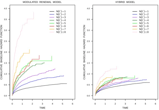
The results of fitting several models of the form (4.1) are reported in Tables 4 and 5. The first model (1A) reported on in Table 4 contains a covariate for sex, a categorical covariate for the cumulative number of prior admissions, which is Ni(t−) for Ni(t−)≤7 and 8 for Ni(t−) ≥8,
and a six-category time-dependent covariate for the time since disease onset. The results reveal a significantly higher rate of admission for women compared to men. We also see a highly significant trend towards increased risk of admission with increasing numbers of prior hospital-izations. There is, however, also a significant trend indicating a lower admission rate with increasing time since first admission (disease on-set). There is evidence of substantial heterogeneity, as represented by the estimate ofϕ.
|
|
|
|
|
|
|
| | | | | | |
− − − − − −
− − − − −
JAN 1, 1994 JAN 1, 1995 JAN 1, 1996 JAN 1, 1997 JAN 1, 1998 JAN 1, 1999 JAN 1, 2000
Bi Ai1Di1 Ai2 Di2 Ai3Di3
Di1 Ai2 Di2 Ai3 Di3
1
2
3
4
5
6
CALEND
AR EFFECT
− − − −
1
2
3
4
5
TIME SINCE DISEASE ONSET
wi1 wi2 wi3
GAP TIMES
Figure 6: Diagram illustrating construction of time-dependent covariates for an individual in the analysis of hospitalizations for affective disorder
To illustrate the effect of omitting the random effect from this model, in Figure 7 we plot the estimated cumulative baseline hazards for the first few gap times based on the corresponding model excluding the random effect (left panel), as well as this model (right panel); here we stratify on the number of prior admissions. As in the simulated example, there is considerably more (spurious) evidence of a trend in the model excluding the random effect than in the model which appropriately accommodates heterogeneity.
The conclusions about the effects of these variables are unchanged when we also adjust for the age of onset (Model 2A). Here we see a sig-nificantly lower rate of admission for those individuals with later ages of onset. The third model (Model 3A) indicates that if we include period of onset but drop years since onset as a factor, the effect of prior admis-sions becomes inconsistent, with negative and then positive effects. This may be because the prior admissions parameters are compensating for the missing years since onset effects; models 1A and 2A indicate
site trends for years since onset (decreasing trend) and number of prior admissions (increasing trend). The final model (4A) includes an effect for both the period of onset and years since onset, and for this we find also a lower rate of re-admission for those individuals with disease onset in the latter part of the observation window, but a consistent pattern for the effect of prior admissions similar to those for models 1A and 2A. For each of these models there remains significant heterogeneity in the admission process across individuals.
Table 5 contains analogous results for models with other time-depend-ent covariates. In these models the age and period variables do not re-late to disease onset but rather are time-dependent covariates indicating current age and current period. The age variable changes at most once during the period of observation given the wide age intervals used, but the period variable changes with each year. The conclusions are broadly similar to those of the analyses reported in Table 4 except that in this case the effect of prior admissions is consistent across all four models. This may be due to the fact that for the third model, the current age and period variables compensate for the missing years since onset, whereas the period of onset variable in Model 3A of Table 4 does not do this.
0 1 2 3 4 5 6
0.0 0.5 1.0 1.5 2.0 2.5 3.0 3.5 4.0
CUMULA
TIVE BASELINE HAZARD FUNCTION
TIME
MODULATED RENEWAL MODEL
N(t−)=1 N(t−)=2 N(t−)=3 N(t−)=4 N(t−)=5 N(t−)=6 N(t−)=7 N(t−)≥8
0 1 2 3 4 5 6
0.0 0.5 1.0 1.5 2.0 2.5 3.0 3.5 4.0
CUMULA
TIVE BASELINE HAZARD FUNCTION
TIME HYBRID MODEL
N(t−)=1 N(t−)=2 N(t−)=3 N(t−)=4 N(t−)=5 N(t−)=6 N(t−)=7 N(t−)≥8
Figure 7: Estimates of cumulative baseline hazards from modulated renewal and hybrid models related to Model 1A of Table 4
T able 4: Results of in tensit y-based analyses of hospital re-admissions among patien ts with affectiv e disorder. MODEL 1A MODEL 2A MODEL 3A MODEL 4A EST SE p EST SE p EST SE p EST SE p Sex: F emale vs. Male 0.101 0.032 0.0018 0.113 0.033 0.0006 0.113 0.035 0.0011 0.111 0.033 0.0008 Prior Admissions (Ref: 1) < 0 . 0001 < 0 . 0001 < 0 . 0001 < 0 . 0001 2 0.049 0.037 0.1933 0.012 0.038 0.7531 -0.133 0.035 0.0002 -0.004 0.038 0.9135 3 0.096 0.054 0.0755 0.042 0.054 0.4377 -0.181 0.047 0.0001 0.024 0.054 0.6629 4 0.273 0.071 0.0001 0.208 0.071 0.0033 -0.069 0.061 0.2598 0.188 0.071 0.0081 5 0.335 0.087 0.0001 0.258 0.087 0.0032 -0.063 0.078 0.4201 0.232 0.087 0.0081 6 0.294 0.111 0.0081 0.209 0.111 0.0607 -0.147 0.101 0.1471 0.189 0.111 0.0888 7 0.631 0.130 < 0 . 0001 0.532 0.131 < 0 . 0001 0.155 0.121 0.2030 0.510 0.131 < 0 . 0001 ≥ 8 0.898 0.090 < 0 . 0001 0.821 0.090 < 0 . 0001 0.404 0.070 < 0 . 0001 0.802 0.091 < 0 . 0001 Y ears Since Disease Onset (Ref: [0 , 1)) 0.0001 0.0004 < 0 . 0001 [1 , 2) -0.009 0.044 0.8407 0.005 0.044 0.9097 -0.023 0.044 0.6117 [2 , 3) -0.222 0.062 0.0004 -0.201 0.062 0.0013 -0.242 0.063 0.0001 [3 , 4) -0.207 0.076 0.0066 -0.180 0.077 0.0184 -0.229 0.077 0.0030 [4 , 5) -0.251 0.095 0.0080 -0.222 0.095 0.0197 -0.274 0.096 0.0044 [5 , ∞ ) -0.472 0.160 0.0031 -0.444 0.160 0.0055 -0.489 0.161 0.0024 Age of Onset (Ref: [0 , 20)) < 0 . 0001 < 0 . 0001 < 0 . 0001 [20 , 40) -0.218 0.096 0.0236 -0.245 0.102 0.0168 -0.234 0.097 0.0162 [40 , 60) -0.374 0.096 < 0 . 0001 -0.429 0.102 < 0 . 0001 -0.405 0.097 < 0 . 0001 [60 , 80) -0.454 0.096 < 0 . 0001 -0.518 0.102 < 0 . 0001 -0.492 0.098 < 0 . 0001 [80 , ∞ ) -0.602 0.109 < 0 . 0001 -0.665 0.115 < 0 . 0001 -0.639 0.110 < 0 . 0001 P erio d of Onset (Ref: [1994 , 1995)) < 0 . 0001 < 0 . 0001 [1995 , 1996) 0.039 0.052 0.4547 0.028 0.050 0.5734 [1996 , 1997) -0.021 0.053 0.6971 -0.038 0.051 0.4615 [1997 , 1998) -0.028 0.053 0.6022 -0.056 0.052 0.2823 [1998 , 1999) -0.144 0.057 0.0121 -0.171 0.056 0.0022 [1999 , 2000) -0.369 0.073 < 0 . 0001 -0.375 0.072 < 0 . 0001 F railt y V ariance 0.637 0.679 0.873 0.682
T able 5: Results of in tensit y-based analyses of hospital re-admissions among patien ts with affectiv e disorder with time-dep enden t age and p erio d effects. MODEL 1B MODEL 2B MODEL 3B MODEL 4B EST SE p EST SE p EST SE p EST SE p Sex: F emale vs. Male 0.101 0.032 0.0018 0.111 0.033 0.0007 0.111 0.033 0.0008 0.110 0.033 0.0008 Prior Admissions (Ref: 1) < 0 . 0001 < 0 . 0001 < 0 . 0001 < 0 . 0001 2 0.049 0.037 0.1933 0.029 0.037 0.4418 0.003 0.035 0.9279 0.051 0.037 0.1760 3 0.096 0.054 0.0755 0.067 0.054 0.2135 0.024 0.047 0.6081 0.104 0.054 0.0562 4 0.273 0.071 0.0001 0.236 0.071 0.0009 0.176 0.062 0.0043 0.281 0.071 < 0 . 0001 5 0.335 0.087 0.0001 0.287 0.087 0.0010 0.205 0.078 0.0084 0.330 0.087 0.0002 6 0.294 0.111 0.0081 0.240 0.111 0.0306 0.156 0.102 0.1261 0.299 0.111 0.0071 7 0.631 0.130 < 0 . 0001 0.561 0.131 < 0 . 0001 0.468 0.122 0.0001 0.623 0.131 < 0 . 0001 ≥ 8 0.898 0.090 < 0 . 0001 0.858 0.090 < 0 . 0001 0.762 0.072 < 0 . 0001 0.932 0.090 < 0 . 0001 Y ears Since Disease Onset (Ref: [0 , 1)) 0.0001 0.0009 0.0204 [1 , 2) -0.009 0.044 0.8407 0.006 0.044 0.8874 0.018 0.044 0.6880 [2 , 3) -0.222 0.062 0.0004 -0.194 0.062 0.0019 -0.165 0.063 0.0092 [3 , 4) -0.207 0.076 0.0066 -0.169 0.077 0.0270 -0.104 0.078 0.1849 [4 , 5) -0.251 0.095 0.0080 -0.208 0.095 0.0287 -0.088 0.098 0.3676 [5 , ∞ ) -0.472 0.160 0.0031 -0.424 0.160 0.0081 -0.251 0.163 0.1236 Age (Ref: [0 , 20)) < 0 . 0001 < 0 . 0001 < 0 . 0001 [20 , 40) -0.159 0.105 0.1300 -0.176 0.106 0.0965 -0.172 0.105 0.1008 [40 , 60) -0.354 0.105 0.0008 -0.389 0.106 0.0002 -0.377 0.105 0.0003 [60 , 80) -0.431 0.106 < 0 . 0001 -0.473 0.107 < 0 . 0001 -0.459 0.106 < 0 . 0001 [80 , ∞ ) -0.497 0.114 < 0 . 0001 -0.540 0.115 < 0 . 0001 -0.525 0.114 < 0 . 0001 P erio d (Ref: [1994 , 1995)) < 0 . 0001 < 0 . 0001 [1995 , 1996) -0.021 0.071 0.7621 -0.031 0.071 0.6595 [1996 , 1997) -0.057 0.069 0.4119 -0.059 0.070 0.3928 [1997 , 1998) -0.065 0.069 0.3433 -0.059 0.069 0.3966 [1998 , 1999) -0.128 0.069 0.0660 -0.118 0.070 0.0903 [1999 , 2000) -0.269 0.070 0.0001 -0.254 0.071 0.0003 F railt y V ariance 0.637 0.652 0.682 0.617
The results in Tables 4 and 5 indicate that the gaps between admis-sions tend to decrease with the number of prior admisadmis-sions, but that this is offset by a tendency for gaps between admissions to increase with calendar time, age and years since disease onset. To examine the differ-ences between individuals with unipolar and bipolar affective disorder, we fitted models analogous to those in Tables 4 and 5 but including a bi-nary time-dependent variable indicating a diagnosis of bipolar disorder. These models reveal a significantly higher re-admission rate following a bipolar diagnosis; for example, adding this variable to Model 1A gives
RR= 1.29 (95% CI: 1.18, 1.41;p <0.0001). The evidence of higher risk of re-admission following a diagnosis of bipolar disorder is present in all fitted models. Similar conclusions are reached from sensitivity analy-ses in which the same models were fit but on a data set excluding an individual with 89 hospital admissions, but these models generally had lower estimates of the frailty variance parameter.
A marginal analysis of the effect of prior admissions, as in Figure 5, is biased towards persons with earlier onset and age of onset, which gives longer periods of followup. Thus, the effects of prior admissions seen in Figure 5 are larger than the relative risks seen in Tables 4 and 5.
5
Discussion
There is a wide variety of models that can be fitted to recurrent event data, and different models lead to different characterizations of trends. It is important that models which allow an assessment of different aspects of trend be considered. As illustrated in Section 4, there may be several types of trend present in data and it can be challenging to distinguish them. We should add that model diagnostics are important but this is challenging when heterogeneity is present and when there is a large number of individuals but small numbers of events per individual. To a large extent, model checking will depend on comparisons with expanded models in which additional structure is present. We have illustrated this to some degree in the application.
An important point that we have not dealt with is selection effects. These arise when patients are included or withdrawn from studies for reasons related to their event processes. In the context of the psychiatry study, patients may die during the course of follow-up and if there is an association between death and the admission process the individuals remaining on study may be at lower risk of admission and re-admission.
This would help explain apparent lower re-admission rates with increas-ing time since disease onset or even calendar/period effects. The plot on the right-hand side of Figure 5 does not suggest a strong relation between admission and death, but this is examined in the context of a marginal Markov model with the time-scale based on age.
The model (3.1) has a parsimonious way of characterizing depen-dence on the event history for a given individual. Gjessing et al. (2010) discuss such models and point out that because of the exponential term exp(βNi(t−)), the model “explodes” ift is allowed to become large. To
avoid this problem, we adopt useful closely related models in the sim-ulation studies and application in which the event count in the linear predictor is capped at some specified value. When this upper limit is reasonably large, trends of this sort can still be effectively studied.
Acknowledgements
Data on psychiatric hospitalizations were kindly provided by Professor Lars Vedel Kessing and Professor Per Kragh Andersen who have used the data in prior publications on recurrent events. This research was supported by the Natural Sciences and Engineering Research Council of Canada (RJC and JFL) and the Canadian Institutes for Health Research (RJC). Richard Cook is a Canada Research Chair in Statistical Methods for Health Research. We thank Ker-Ai Lee for programming assistance in the simulation studies.
Appendix: Derivation of (3.3)
Assume the historyHi(t) consists ofn−1 events, at timesti1, . . . , ti,n−1. Writing “Pr” to denote a probability density for convenience and using (2.11), we find for model (3.1) that
Pr(Hi(t), αi) =
n∏−1
j=1
αih0(Bi(tij))eβ(j−1)
×exp
{
−αi ∫ t
0
h0(Bi(u))eβNi(u
−)
du
}
g(αi)
= αni−1
n∏−1
j=1
h0(wij)eβ(j−1)
×