247
A cross entropy algorithm for continuous covering
location problem
Seyed Javad Hosseininezhad
1*, mohammad Saeed jabalameli
2marjan pesaran haji abbas
11Department of Industrial Engineering, K. N. Toosi University of Technology, Tehran, Iran 2School of Industrial engineering, Iran University of Science and Technology, Tehran, Iran
[email protected], [email protected]
Abstract
Covering problem tries to locate the least number of facilities and each demand has at least one facility located within a specific distance. This paper considers a cross entropy algorithm for solving the mixed integer nonlinear programming (MINLP) for covering location model. The model is solved to determine the best covering value. Also, this paper proposes a Cross Entropy (CE) algorithm considering multivariate normal density function for solving large scale problems. For showing capabilities of the proposed algorithm, it is compared with GAMS. Finally, a numerical example and a case study are expressed to illustrate the proposed model. For case study, Tehran's special drugstores consider and determine how to locate 7 more drugstores to cover all 22 districts in Tehran.
Keywords: Continuous covering location problem (CCLP), uncertainty, cross entropy (CE)
1-Introduction
Covering problem is to locate a set of new facilities such that customers can receive service by each facility if the distance between the customer and the facility is equal or less than a predefined number. This critical value is called coverage. Church and ReVelle (1974) modeled the maximization covering problem. Covering problems are divided into two problems; Total covering and partial covering problems, based on covering all or some demand points. The total covering problem is modeled by Toregas (1971). Up to the present time many developments have occurred about total covering and partial covering problems in solution technique and assumptions. Covering problem has many applications such as: designing of switching circuits, data retrieving, assembly line balancing, airline staff scheduling, locating defend networks, distributing products, warehouse locating, location emergency service facility (Francis et al. 1992). Some researchers investigated network covering problems such as Church and ReVelle (1974), Schilling et al. (1993), Owen and Daskin (1998) and Drezner and Wesolowsky (1999).
By reviewing literature of the covering location models, it be seen that these problems have been investigated in discrete space, only. While there are some cases in real world which may be occurred in continuous space, we introduce a continuous covering location problem in this paper; we are interested in finding the location of k facilities in continuous space in order to serve customers at n
demand points so that the total cost of installation facilities sites and uncovered customers are minimized.
*Corresponding author
ISSN: 1735-8272, Copyright c 2018 JISE. All rights reserved
Journal of Industrial and Systems Engineering Vol. 11, No. 3, pp. 247-260
248
The continuous covering location problem could be used for electronic service facilities like BTS towers or Wi-Fi centers, Aircraft refueling problems and robotics areas (Plaster , 1995).
The reminder of the paper is organized as follows; in section2 a literature review about uncertainty in covering location model are provided. In section 3 we present the mathematical model. Solution approach proposing CE algorithm and based on α- cut method is provided in section4. In section5, a numerical example and case study are given to illustrate the usability of proposed model. Finally, Section6 draws the conclusions and future works.
2-Literature review
In this section, review literature of covering problems and uncertain location models are provided.
Liu et al. (2010) presented a location model that assigns online demands to the capacitated regional warehouses currently serving in-store demands in a multi-channel supply chain. The model explicitly considered the trade-off between the risk pooling effect and the transportation cost in a two-echelon inventory/logistics system. They formulated the assignment problem as a non-linear integer programming model. A strategic supply chain management problem was studied by Peng et al. (2011) to design reliable networks that perform as well as possible under normal conditions, while also performing relatively well when disruptions strike. They presented a mixed-integer programming model whose objective was to minimize the nominal cost while reducing the uncertainty using the p -robustness criterion which bounds the cost in disruption scenarios. Chen et al. (2011) presented a multi-criteria decision analysis for environmental uncertainty assessment with regard to avoiding and eliminating damages and loss under natural disasters in international airport projects. They used the ANP to demonstrate one of its utility modes in decision making support to location selection problems, which aims at an evaluation of different projects from different locations. A corresponding framework for value-based performance and uncertainty optimization in a single-stage supply chain problem was developed by Hahn and Kuhn (2012). They applied Economic Value Added as a prevalent metric of value-based performance to mid-term sales and operations planning. Due to the uncertainty of future events in a scenario based problem, they also used robust optimization methods to deal with operational risks in physical and financial supply chain management. Nickel S. et al (2012) provided a multi-period supply chain network design problem. In this problem, uncertainty was assumed for demand and interest rates, which was described by a set of scenarios. Accordingly, the problem was formulated as a multi-stage stochastic mixed-integer linear programming problem. Hosseininezhad et al. (2013) proposed a continuous covering location model with risk consideration. Because the model considered uncertain covering radius, fuzzy concept introduced for customer satisfaction degree of covering. The model is solved by a fuzzy method named a-cut. After solving the model, the zones with the largest possibilities are determined for locating new facilities. Mohammadi et al. (2013) developed multi-objective multi-mode transportation model for hub covering location problem under uncertainty. In this model, uncertain parameter is the transportation time between each pair of nodes and it influence by a risk factor in the network. Akgun et al (2014) developed a model that minimizes the risk of demand point that is not supported by the located facilities. The goal is to choose the locations to support the demand points is constructed. In this paper, the uncertainty of demand point is calculated as the multiplication of the threat, the vulnerability of the demand point and consequence. Zhang et al. (2016) investigated a facility location model that considered the disruptions of facilities and the cost savings from the inventory risk-pooling effect and economies of scale. Facilities might have heterogeneous disruption probabilities. When a facility failed, its customers may be re-assigned to other ones that survive, to hedge against lost-sales costs. Puga and Tancrez (2016) studied on a location-inventory problem for the design of large networks with uncertain demand. They defined a non-linear formulation that integrates location, allocation and inventory decisions, and also includes the costs of transportation, cycle inventory, safety stock, ordering and facility opening. Berman et al. (2016) studied the effect of a decision maker's risk attitude on the median and center problems, with uncertain demand in the mean variance framework. They provided a mathematical formulation for both types in the form of quadratic programming. Lutter et al. (2017) introduced robust optimization and set covering problem by combining robust and probabilistic optimization. They defined new constraint and for highlighting their new approach, a case study for the location of emergency services was introduced.
249
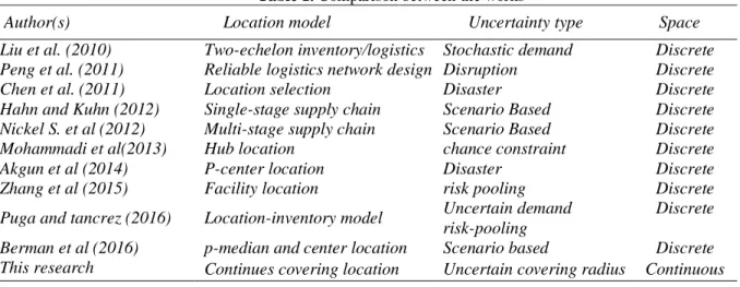
In the rest of this section, aforementioned articles are classified based on location model, uncertainty and space as shown in Table 1 in order to help the reader appreciate the symmetry associated with the facility location problems.
Table 1. Comparison between the works
In the next section, a continuous covering model with uncertainty consideration is introduced. The model is solved to determine the best covering value. Also, this paper proposes a CE algorithm considering multivariate normal density function for solving large scale problems.
3-Continuous covering location problem (CCLP)
In this section, the continuous covering model based on the hosseininezhad et al. (2013) is considered. For this model, the space is divided into n zones as shown in Error! Reference source not found.. Two new variables 𝑧𝑗𝑖 and 𝑢𝑗𝑖 are also introduced in this model. 𝑧𝑗𝑖 shows whether
facility j is located in zone i ornotand𝑢𝑗𝑖 shows whether customer i is covered by facility j or not. It
is assumed that distance between each customer and the facility is Euclidean. Accordingly, the mixed integer nonlinear programming model 𝑃2 is as follows:
( 5 )
𝑚𝑖𝑛 ∑ ∑ 𝑧𝑗𝑖𝑓𝑖
𝑛
𝑖=1 𝑘
𝑗=1
+ 𝑀 ∑ (𝐶𝑖
𝐶) 𝑛 𝑖=1 𝑞𝑖 S.t. ( 6 )
(√(𝑥𝑗−𝑎𝑖)
2
+ (𝑦𝑗−𝑏𝑖)
2
) ≤ 𝑅 + 𝐿(1 − 𝑢𝑗𝑖), ∀𝑖 = 1,2, … , 𝑛, ∀𝑗 = 1,2, … , 𝑘
( 7 )
(√(𝑥𝑗−𝑎𝑖)
2
+ (𝑦𝑗−𝑏𝑖)
2
) ≥ 𝑅 − 𝐿𝑢𝑗𝑖, ∀𝑖 = 1,2, … , 𝑛, ∀𝑗 = 1,2, … , 𝑘
( 8 )
∑ 𝑢𝑗𝑖
𝑘
𝑗=1
+ 𝑞𝑖≥ 1, 𝑖 = 1,2, … , 𝑛
( 9 )
∑ 𝑧𝑗𝑖
𝑛
𝑖=1
(√(𝑥𝑗−𝑎𝑖)
2
+ (𝑦𝑗−𝑏𝑖)
2
) ≤ 𝐷, ∀𝑗 = 1,2, … , 𝑘
(10)
∑ 𝑧𝑗𝑖
𝑛
𝑖=1
= 1, ∀𝑗 = 1,2, … , 𝑘
( 11 )
∑ 𝑧𝑗𝑖
𝑘
𝑗=1
≤ 1, ∀𝑖 = 1,2, … , 𝑛
Space Uncertainty type Location model Author(s) Discrete Stochastic demand Two-echelon inventory/logistics Liu et al. (2010)
Discrete Disruption
Reliable logistics network design Peng et al. (2011)
Discrete Disaster
Location selection Chen et al. (2011)
Discrete Scenario Based
Single-stage supply chain Hahn and Kuhn (2012)
Discrete Scenario Based
Multi-stage supply chain Nickel S. et al (2012)
Discrete chance constraint
Hub location Mohammadi et al(2013)
Discrete Disaster
P-center location Akgun et al (2014)
Discrete risk pooling
Facility location Zhang et al (2015)
Discrete Uncertain demand
risk-pooling Location-inventory model
Puga and tancrez (2016)
Discrete Scenario based
p-median and center location Berman et al (2016)
Continuous Uncertain covering radius
Continues covering location This research
250
( 12 )
∑ ∑ 𝑧𝑗𝑖
𝑛
𝑖=1 𝑘
𝑗=1
≤ 𝑃,
Notations of the model are as follows, Description Notations
Sets/Indices
set of zones(customer) in a continuous space indexed by i ,
{i=1,2,…,n}
Nset of new facilities to be located indexed by j,
{j=1,2,…,k}
KParameters
x coordinate of customer i 𝑎𝑖
y coordinate of customer i 𝑏𝑖
Installation cost of each facility in zone i 𝑓𝑖
Maximum distance a facility could be located from center of a zone for belonging to the zone
𝐷
Maximum distance a customer could be located from a facility to be covered by the facility (covering radius)
𝑅
importance of customer i 𝐶𝑖
Overall importance of customers 𝐶
Penalty of uncovered customers which is a large value M
a large value L
Number of facilities that can be open 𝑃
Decision variable
x coordinate of facility j 𝑥𝑗
y coordinate of facility j 𝑦𝑗
Binary variable; equal to1 if facility j is located in zone i; equal to 0 otherwise 𝑧𝑗𝑖
Binary variable; equal to 1 if customer i is covered by facility j; equal to 0 otherwise;
𝑢𝑗𝑖
Binary variable; equal to 1 if customer i is not covered; equal to 0 otherwise 𝑞𝑖
Equation (5) is objective function of the model 𝑃2 and constitutes of two terms; the first term is
installation cost and the second term is risk cost which is cost of uncovered customers based on importance of each customer. Constraint sets (6), (7) are covering constraints; Guarantee that each customer can be covered by a facility if distance between them is smaller than 𝑅; 𝑢𝑗𝑖’s (∀𝑖 =
1,2, … , 𝑛 𝑎𝑛𝑑 ∀𝑗 = 1,2, … , 𝑘) constitute covering matrix. If distance between customer i and facility j
is greater than 𝑅 then 𝑢𝑗𝑖= 0 and 𝑢𝑗𝑖 = 1 otherwise; since L is a large value Constraint sets (6), (7)
will be satisfied, simultaneously. Constraint set (8) indicates the demand constraint which guarantees that 𝑞𝑖 is 1 if 𝑢𝑗𝑖 is zero, it means that customer i is not covered. Constraint set (9) guarantees if
distance between facility j and zone i is greater than D, 𝑧𝑗𝑖 = 0, so facility j does not belong to zone i
and facility j will be located in zone i, if distance between facility j and zone i is smaller than D,
Constraint set (10) Guarantees that facility j is installed only in one zone. Constraint set (11) Guarantees that at most one facility could be located in zone i. constraint set (12) defines number of facilities that should be open.
4-Solution method
In this section a solution method based on Cross Entropy (CE) algorithm is proposed
.
4-1- Cross entropy (CE) algorithm
The main idea of CEalgorithm, which was introduced by Rubinstein (1997), is related to the design of an effective learning mechanism throughout the search. It associates an estimation problem to the
251
original combinatorial optimization problem, called the associated stochastic problem, characterized by a density function 𝜙. The stochastic problem is solved by identifying the optimal importance sampling density 𝜙∗, which is the one that minimizes the Kullback-Leibler distance with respect to the original density 𝜙. This distance is also called the CE between 𝜙 and𝜙∗. The minimization of the
CE leads to the definition of optimal updating rules for the density functions, and consequently to the generation of improved feasible vectors. The method terminates when convergence to a point in the feasible region is achieved. The most important features of CE algorithm have been thoroughly exposed by de Boer et al. (2005). Chepuri and Homem-de-Mello (2005) considered CE algorithm to solve the vehicle routing problem with stochastic demands. Sebaa et al (2014) solved the location and tuning problems with cross entropy approach and compared the performance of CE algorithm with genetic algorithm. In this paper, we present a CE algorithm to solve CCLP. Since we want to generate vectors to identify the location of each facility, a density functions is considered. Consequently, let us define a family of density function 𝜙 on X, and use 2-dimensional multivariate normal density function for locating facilities under the following probability distribution function:
( (4 )
𝜙(𝑋, 𝜇, Σ) = 𝑒
−(𝑋−𝜇)Σ−1(𝑋−𝜇)𝑇⁄21
Σ
1 2⁄2𝜋
⁄
Where X=(x,y) and 𝜇 = (𝜇𝑥, 𝜇𝑦) are 1-by-2 vectors x , y coordinates of facility locations and mean
of feasible space and Σ is a 2-by-2 symmetric positive definite matrix covariance. We estimate X via
Monte Carlo simulation. In this regard, 𝑋 could be estimated by drawing a random sample 𝑋1, … , 𝑋𝑃−𝑠𝑖𝑧𝑒 from 𝜙(𝑋, 𝜇, Σ), where P-size is CE population size, after generation each one of
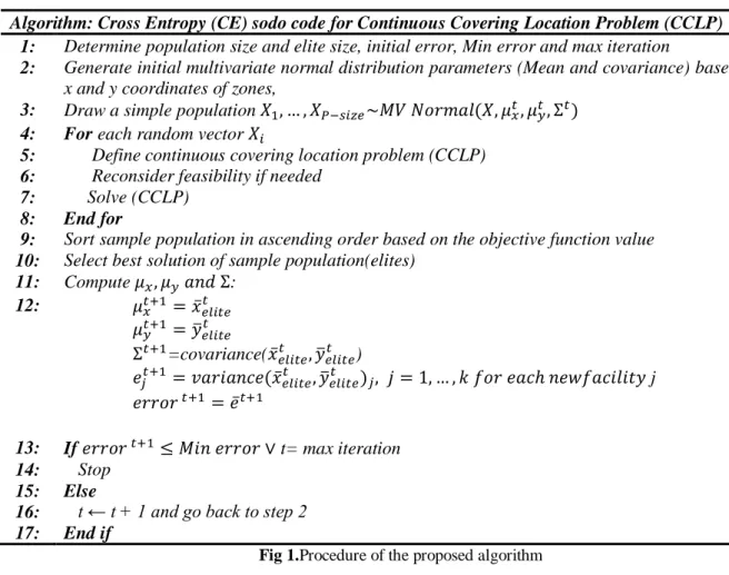
iterations, the best solutions (elites) are selected to constitute new space solution. Figure 1 shows the procedure of the algorithm.
In the following, we provide the CE procedure for CCLP as pseudo-code. As illustrated in step13, the algorithm terminates when either the variance of multivariate normal density function converges to a small value (Min error) or when a pre-fixed maximum number of iteration (max iteration) is reached.
Fig 1.Procedure of the proposed algorithm
Algorithm: Cross Entropy (CE) sodo code for Continuous Covering Location Problem (CCLP) 1: Determine population size and elite size, initial error, Min error and max iteration
2: Generate initial multivariate normal distribution parameters (Mean and covariance) based on x and y coordinates of zones,
3: Draw a simple population 𝑋1, … , 𝑋𝑃−𝑠𝑖𝑧𝑒~𝑀𝑉 𝑁𝑜𝑟𝑚𝑎𝑙(𝑋, 𝜇𝑥𝑡, 𝜇𝑦𝑡, Σ𝑡)
4: For each random vector 𝑋𝑖
5: Define continuous covering location problem (CCLP)
6: Reconsider feasibility if needed
7: Solve (CCLP)
8: End for
9: Sort sample population in ascending order based on the objective function value
10: Select best solution of sample population(elites)
11: Compute 𝜇𝑥, 𝜇𝑦 𝑎𝑛𝑑 Σ:
12: 𝜇𝑥𝑡+1 = 𝑥̅𝑒𝑙𝑖𝑡𝑒𝑡
𝜇𝑦𝑡+1 = 𝑦̅𝑒𝑙𝑖𝑡𝑒𝑡
Σ𝑡+1=covariance(𝑥̅
𝑒𝑙𝑖𝑡𝑒𝑡 , 𝑦̅𝑒𝑙𝑖𝑡𝑒𝑡 )
𝑒𝑗𝑡+1= 𝑣𝑎𝑟𝑖𝑎𝑛𝑐𝑒(𝑥̅𝑒𝑙𝑖𝑡𝑒𝑡 , 𝑦̅𝑒𝑙𝑖𝑡𝑒𝑡 )𝑗, 𝑗 = 1, … , 𝑘 𝑓𝑜𝑟 𝑒𝑎𝑐ℎ 𝑛𝑒𝑤𝑓𝑎𝑐𝑖𝑙𝑖𝑡𝑦 j
𝑒𝑟𝑟𝑜𝑟 𝑡+1= 𝑒̅𝑡+1
13: If𝑒𝑟𝑟𝑜𝑟 𝑡+1≤ 𝑀𝑖𝑛 𝑒𝑟𝑟𝑜𝑟∨ t= max iteration
14: Stop
15: Else
16: t ← t + 1 and go back to step 2
252
4-2- Computational results
In this section, we present results of applying the CE algorithm on some instances of the continuous covering location problem. The algorithm has been implemented in Matlab, and run on a Corei5 at 2.53 GHz with 3GB of RAM memory. The CE parameters are as follows; the population size is 250
and the elite size is 25. We compare obtained CPU time and objective value of the proposed algorithm with GAMS software which is solved by SBB (Simple Branch & Bound) solver (baron solver-12). These results are expressed as a percent deviation from the best-known solutions by GAMS. The deviation is computed as follows:
(15) 𝑑𝑒𝑣. =𝐹
𝑏𝑒𝑠𝑡− 𝐹∗
𝐹∗ × 100
Where Fbest is the total cost found by the proposed algorithm, and F* refers to the best found by
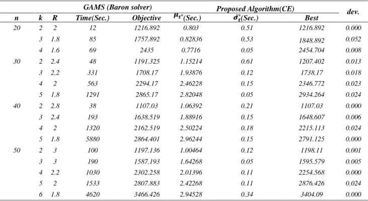
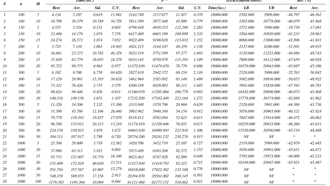
GAMS. We ran the algorithms ten times for each instance and report the following statistics based on the best solutions. As shown in table 2 the proposed method provides better solution and smaller CPU Time. For all of the problems, the gap for gams is 0.01. Note CPU time for GAMS to provide a feasible solution is very high for n>50 & k>5. Then the algorithm has been solved for large scale cases until n=1000 and k=100. Figure 2 and figure 3 show objective function vs. iteration and location of facilities for n=500 and k=50. Table 3 provides results for large scale cases.
Table 2.Comparision between results of the Proposed Algorithm(CE) and GAMS solution
GAMS (Baron solver) Proposed Algorithm(CE)
dev. n k R Time(Sec.) Objective *(Sec.) **(Sec.) Best
20 2 2 12 1216.892 0.803 0.51 1216.892 0.000
3 1.8 85 1757.892 0.82836 0.53 1848.892 0.052
4 1.6 69 2435 0.7716 0.05 2454.704 0.008
30 2 2.4 48 1191.325 1.15214 0.61 1207.402 0.013
3 2.2 331 1708.17 1.93876 0.12 1738.17 0.018
4 2 563 2294.17 2.46228 0.15 2346.772 0.023
5 1.8 1291 2865.17 2.82048 0.05 2934.264 0.024
40 2 2.8 38 1107.03 1.06392 0.21 1107.03 0.000
3 2.4 193 1638.519 1.88916 0.15 1648.607 0.006
4 2 1320 2162.519 2.50224 0.18 2215.113 0.024
5 1.8 5880 2864.401 2.96244 0.15 2791.125 0.000
50 2 3 100 1197.136 1.00464 0.12 1198.11 0.001
3 3 190 1587.193 1.64268 0.05 1595.579 0.005
4 2.2 1030 2302.258 2.01396 0.11 2254.568 0.000
5 2 1533 2807.883 2.42268 0.11 2876.426 0.024
6 1.8 4620 3466.426 2.94528 0.34 3404.09 0.000
*Average Time over 10 runs
253
Table 3. Results of the proposed algorithm (CE) for large scale problems
# n M Time(Sec.) F
best GAMS(Baron solver) dev. (%)
Best Avr. Std. C.V. Best Avr. Std. C.V. Time(Sec.) LB UB Best Avr.
1 100 5 4.134 5.187 0.619 11.941 3143.748 3157.677 11.927 0.378 18000.000 2582.000 5909.000 -46.797 -46.562 2 100 10 18.798 30.379 10.549 34.726 5811.589 5877.440 45.800 0.779 18000.000 5305.000 10778.000 -46.079 -45.468 4 150 5 4.555 5.524 0.531 9.605 4798.448 4958.553 112.290 2.265 18000.000 2571.000 5980.000 -19.758 -17.081 5 150 10 12.496 14.179 1.074 7.576 6417.408 6665.189 168.988 2.535 18000.000 5264.000 10920.000 -41.233 -38.963 6 150 15 24.274 26.573 1.874 7.052 9022.489 9190.628 115.032 1.252 18000.000 8060.000 15800.000 -42.896 -41.831 7 200 5 5.725 7.110 1.063 14.945 3021.215 3144.107 48.359 1.538 18000.000 2537.000 6280.000 -51.891 -49.935 8 200 10 16.661 23.273 10.782 46.329 5623.519 5751.599 97.277 1.691 18000.000 5129.000 11221.000 -49.884 -48.743 9 200 15 37.830 65.779 16.035 24.378 8433.145 8550.979 115.393 1.349 18000.000 7809.000 16112.000 -47.659 -46.928 10 200 20 95.722 98.575 0.963 0.977 11372.650 11479.670 78.770 0.686 18000.000 10579.000 20943.000 -45.697 -45.186 11 300 5 6.162 9.706 6.758 69.620 2827.619 2942.572 68.154 2.316 18000.000 2528.000 5986.000 -52.763 -50.842 12 300 10 17.129 29.991 15.193 50.658 5461.964 5585.892 83.149 1.489 18000.000 5082.000 10936.000 -50.055 -48.922 13 300 15 73.321 76.426 2.735 3.579 8300.199 8428.803 88.111 1.045 18000.000 7693.000 15838.000 -47.593 -46.781 14 300 20 98.624 99.446 0.826 0.831 11160.670 11285.864 100.778 0.893 18000.000 10342.000 20696.000 -46.073 -45.468 15 300 30 146.516 149.156 1.651 1.107 17232.920 17542.449 223.164 1.272 18000.000 15778.000 30174.000 -42.888 -41.862 16 500 5 11.326 14.506 2.232 15.386 3333.048 3370.796 20.904 0.620 18000.000 2528.000 5991.000 -44.366 -43.736 17 500 10 31.590 45.786 12.106 26.440 5863.962 5940.348 54.154 0.912 18000.000 5076.000 10965.000 -46.521 -45.824 18 500 15 70.778 110.393 19.837 17.970 8518.412 8583.694 52.623 0.613 18000.000 7647.000 15914.000 -46.472 -46.062 19 500 20 96.580 153.011 20.213 13.210 11174.810 11326.646 76.033 0.671 18000.000 10259.000 20833.000 -46.360 -45.631 20 500 30 224.158 230.833 3.859 1.672 16665.630 16980.993 221.816 1.306 18000.000 15550.000 30590.000 -45.519 -44.488
21 500 50 384.511 387.017 2.788 0.720 28754.280 29243.232 238.276 0.815 18000.000 NF NF * *
22 1000 5 25.584 29.600 3.718 12.562 3420.706 3452.719 25.105 0.727 18000.000 2519.000 5999.000 -42.979 -42.445 23 1000 10 57.096 65.311 5.921 9.065 5973.489 6103.208 82.572 1.353 18000.000 5050.000 10991.000 -45.651 -44.471 24 1000 15 95.753 121.007 19.779 16.346 8625.463 8747.928 82.899 0.948 18000.000 7595.000 15973.000 -46.000 -45.233 25 1000 20 131.400 172.810 40.630 23.511 11327.830 11418.793 82.323 0.721 18000.000 10149.000 20947.000 -45.921 -45.487
26 1000 30 291.784 357.567 43.905 12.279 16818.600 17022.362 132.108 0.776 18000.000 NF NF * *
27 1000 50 548.359 588.955 17.156 2.913 28394.870 28561.002 160.145 0.561 18000.000 NF NF * *
254
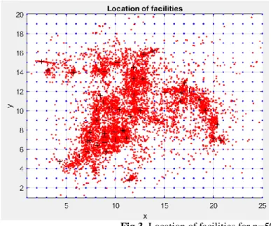
Fig 2.Objective function vs. iteration for n=500 and k=50
Solution in different iterations
Location of customers
Location of facilities
Fig 3. Location of facilities for n=500 and k=50 Sensitivity analysis for parameter M and L are shown in figure 4 and figure 5.
Fig 4. sensitivity analysis of parameter M
1800 1850 1900 1950 2000
500 1000 1500 2000 2500
o
bjec
ti
ve
func
ti
o
n
M
255
Fig 5. Sensitivity analysis of parameter L
5-Numerical example and case study
In this section, a numerical example is expressed to illustrate the introduced model.
5-1- Example
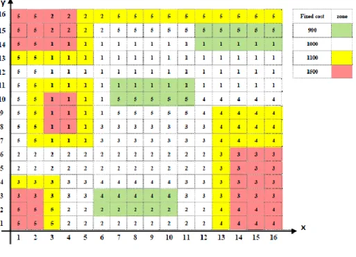
Suppose we want to locate 25 new facilities in a region including 256 zones (customers) as shown infigure 6. Numbers in each region express importance of each customer from 1 to 5. Fixed cost in green, white, yellow and red zones are 900, 1000, 1100 and 1500, respectively.
Fig 6.Example with 256 zones
Inthis example, some neighborhood zones with the same fixed cost are selected as a zone set. For example zone 25 and 38 are selected as zone set {25, 38}.
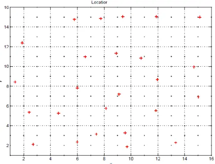
Coordinates of new facilities based on possibility values applying (19) and (20), and cost values for the numerical example 2 are shown in table 4.
1800 1850 1900 1950 2000
R 2*R 3*R 4*R
o
bjec
ti
ve
func
ti
o
n
L
256
Table 4.Coordinate of new facilities based on possibility values for Example Facility Coordinate x Coordinate y
1 2.70 2.10
2 5.98 2.35
3 11.85 5.52
4 15.03 6.91
5 5.99 7.83
6 15.12 14.99
7 2.40 5.36
8 9.70 1.88
9 5.78 14.77
10 1.89 12.40
11 11.95 8.67
12 14.71 9.95
13 11.89 15.06
14 1.34 8.43
15 13.33 2.29
16 4.59 5.26
17 8.90 11.33
18 8.14 5.76
19 10.73 10.84
20 9.38 15.05
21 9.55 3.27
22 9.11 7.19
23 7.75 14.84
24 6.59 10.98
25 7.41 3.14
The final solution is shown infigure 7.
Location of customers
Location of facilities
Fig 7. Results of the numerical example
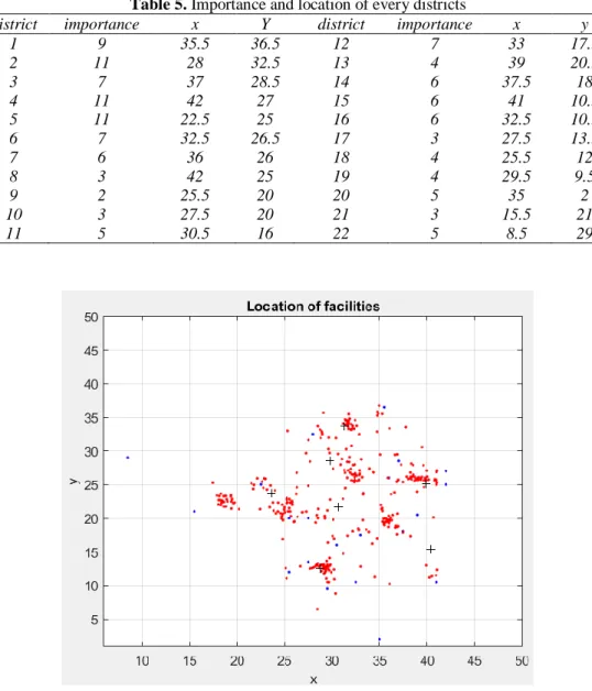
5-2- Case study
In Tehran city, that contains 22 districts, there are 15 special drugstores which service people for their special kinds of medicines. Now, one problem is that these drugstores could be able to service more than one district and cover more districts. The goal is to service quickly, so, we locate 7 new drugstores in Tehran with continuous covering location model with fixed cost.
257
Tehran contains 22 districts and we want to locate 7 new drugstores in these districts. For solving problem, we divided space to 2-dimensional horizontal and vertical. The vertical dimension consider from 0 to 41 and horizontal dimension consider from 0 to 55. Now location of every district is available. In this problem, importance of every district determine with condition and number of service office in that district. Location and importance of every district is shown in table 5. The problem is solved by cross entropy
Table 5. Importance and location of every districts
district importance x Y district importance x y
1 9 35.5 36.5 12 7 33 17.5
2 11 28 32.5 13 4 39 20.5
3 7 37 28.5 14 6 37.5 18
4 11 42 27 15 6 41 10.5
5 11 22.5 25 16 6 32.5 10.5
6 7 32.5 26.5 17 3 27.5 13.5
7 6 36 26 18 4 25.5 12
8 3 42 25 19 4 29.5 9.5
9 2 25.5 20 20 5 35 2
10 3 27.5 20 21 3 15.5 21
11 5 30.5 16 22 5 8.5 29
Fig 8. Location of new 7 drugstores
Figure 8 shows one of solutions. Location of every drug store is shown in table 6. Table 6. possibility of districts and service offices
Selected location
y x districts Services office
14 15.3 40.3 14,15 1
17 12.5 28.7 11,16,17,18,19 2
10 21.62 30.6 10,12 3
2 33.73 31.3 1,2 4
5 23.7 23.6 5,9 5
8 25 39.8 3,4,7,8,13 6
258
With considering the final solution districts of 20, 21 and 22 is not covering and: Drug store that located in district 14, cover a districts 14 and 15.
Drug store that located in district 17, cover a districts 11, 16, 17, 18, 19. Drug store that located in district 10, cover districts 10 and12
Drug store that located in district 2, cover districts 1 and 2. Drug store that located in district 5, cover districts 5 and 9. Drug store that located in district 8, cover districts 3, 4, 7, 8, 13. Drug store that located in district 6, cover districts 2 and 6.
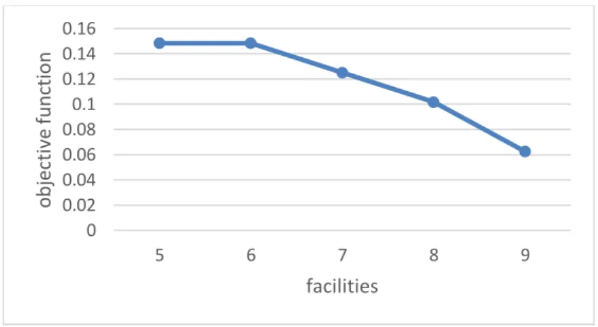
For analysis of case study, 3 parameters consider. The number of facilities, covering radius and Maximum distance a facility could be located from the center of a zone. Figure 9and10show how changing each of these parameters, influence the objective function of the model. As shown in figure 7, considering more facilities reduces the objective function. For the parameter of covering radius, by increasing the covering radius, the objective function decreases and this is shown in figure 8.
Fig 9. sensitivity analysis of parameter number of facilities
Fig 10.sensitivity analysis of parameter covering radius
6-Conclusion
This paper considered the cross entropy algorithm for solving the covering location model. The presented model’s advantage over the traditional covering location ones was consideration of continuous space for the covering problems. Providing robust uncertainty location model is another usability of the proposed model. Comparing with the GAMS, the proposed algorithm based on CE
provided more acceptable results in CPU time and the objective value, especially in large scale problems. The case study showed how to cover demand of 22 districts in Tehran with more 7 new service offices. Also, the location of these facilities is demonstrated by the model. Extension of the
0 0.02 0.04 0.06 0.08 0.1 0.12 0.14 0.16
5 6 7 8 9
o
bjec
ti
ve
func
ti
o
n
facilities
0 0.02 0.04 0.06 0.08 0.1 0.12 0.14 0.16
0 0.5 1 1.5 2
o
bjec
ti
ve
func
ti
o
n
259
model as a continuous covering location allocation model and providing a heuristic method are two research issues which we think may need future investigations.
References
Akgün, İ., Gümüşbuğa, F., & Tansel, B. (2015). Risk based facility location by using fault tree analysis in disaster management. Omega, 52, 168-179.
Berman, O., Sanajian, N., & Wang, J. (2017). Location choice and risk attitude of a decision maker. Omega, 66, 170-181.
Chen, Z., Li, H., Ren, H., Xu, Q., & Hong, J. (2011). A total environmental risk assessment model for international hub airports. International Journal of project management, 29(7), 856-866.
Chepuri, K., & Homem-De-Mello, T. (2005). Solving the vehicle routing problem with stochastic demands using the cross-entropy method. Annals of Operations Research, 134(1), 153-181.
Church, R., & ReVelle, C. (1974, December). The maximal covering location problem. In Papers of
the Regional Science Association (Vol. 32, No. 1, pp. 101-118). Springer-Verlag.
De Boer, P. T., Kroese, D. P., Mannor, S., & Rubinstein, R. Y. (2005). A tutorial on the cross-entropy method. Annals of operations research, 134(1), 19-67.
Hahn, G. J., & Kuhn, H. (2012). Value-based performance and risk management in supply chains: A robust optimization approach. International Journal of Production Economics, 139(1), 135-144.
Drezner, Z., & Wesolowsky, G. O. (1999). Allocation of discrete demand with changing costs. Computers & operations research, 26(14), 1335-1349.
Hosseininezhad, S. J., Jabalameli, M. S., & Naini, S. G. J. (2013). A continuous covering location model with risk consideration. Applied Mathematical Modelling, 37(23), 9665-9676.
Liu, K., Zhou, Y., & Zhang, Z. (2010). Capacitated location model with online demand pooling in a multi-channel supply chain. European Journal of Operational Research, 207(1), 218-231.
Lutter, P., Degel, D., Büsing, C., Koster, A. M., & Werners, B. (2017). Improved handling of uncertainty and robustness in set covering problems. European Journal of Operational Research, 263(1), 35-49.
Mohammadi, M., Jolai, F., & Tavakkoli-Moghaddam, R. (2013). Solving a new stochastic multi-mode p-hub covering location problem considering risk by a novel multi-objective algorithm. Applied
Mathematical Modelling, 37(24), 10053-10073.
Nickel, S., Saldanha-da-Gama, F., & Ziegler, H. P. (2012). A multi-stage stochastic supply network design problem with financial decisions and risk management. Omega, 40(5), 511-524.
Owen, S. H., & Daskin, M. S. (1998). Strategic facility location: A review. European journal of operational research, 111(3), 423-447.
Peng, P., Snyder, L. V., Lim, A., & Liu, Z. (2011). Reliable logistics networks design with facility disruptions. Transportation Research Part B: Methodological, 45(8), 1190-1211.
Plastria, F. (1995). Continuous location problems: research, results and questions. Facility location: a
survey of applications and methods, 85-127.
Puga, M. S., & Tancrez, J. S. (2017). A heuristic algorithm for solving large location–inventory problems with demand uncertainty. European Journal of Operational Research, 259(2), 413-423.
260
Rubinstein, R. Y. (1997). Optimization of computer simulation models with rare events. European
Journal of Operational Research, 99(1), 89-112.
Sebaa, K., Bouhedda, M., Tlemcani, A., & Henini, N. (2014). Location and tuning of TCPSTs and SVCs based on optimal power flow and an improved cross-entropy approach. International Journal of Electrical Power & Energy Systems, 54, 536-545.
Schilling, D. A. (1993). A review of covering problems in facility location. Location Science, 1, 25-55.
Toregas, C., Swain, R., ReVelle, C., & Bergman, L. (1971). The location of emergency service facilities. Operations research, 19(6), 1363-1373.
White, J. A., Francis, R. L., Francis, R. L., & McGinnis, L. F. (1974). Facility layout and location: an analytical approach. Prentice-Hall.
Zhang, Y., Snyder, L. V., Qi, M., & Miao, L. (2016). A heterogeneous reliable location model with risk pooling under supply disruptions. Transportation Research Part B: Methodological, 83, 151-178.