Thesis

Validation of spatiotemporal image correlation spectroscopy (STICS) for the measurement of diffusion

By

Pranav Haravu

Senior Honors Thesis

Quantitative Biology (B.S.)

University of North Carolina at Chapel Hill

4/14/16

Approved:

________________________

Michael Falvo, Thesis Advisor

Mark Peifer, Reader

Steve Rogers, Reader

This thesis has been prepared in conjunction with BIOL692H and in partial satisfaction

ABSTRACT

Understanding of chemical mechanisms on an intracellular level is steadily

growing and extensively studied. However, our understanding of the physical bases for

these processes is comparatively lacking. Current limitations on measuring fundamental

intranuclear mechanical properties have stifled necessary new perspectives on

intranuclear mechanics. Here we build on the Wiseman group’s novel development of

spatiotemporal image correlation spectroscopy (STICS) to measure diffusion, and then

attempt to validate it with simulated and experimental datasets. STICS, unlike current

methods of diffusion measurement, such as image mean square displacement (iMSD),

does not require the ability to track distinct particles. Expected diffusion coefficients, D,

in simulated datasets were calculated using the Stokes-Einstein relation, which relates the

diffusive properties of particles moving in fluids as D= kBT

6πηr . For experimental bead

diffusion datasets expected D values were measured using iMSD. We observe that in

simulated datasets STICS is able to measure a linear relationship between 1/D and the

viscosity, η, as expected by Stokes-Einstein. We also see that STICS has a high

precision, as D measured from subsamples of a given video have an average standard

deviation of 3.23×10−14_m2_/s

. However, in both simulated and experimental datasets the

measured D value, denoted DS , differs from the expected D by a calibration factor

D=βDS that appears to depend on particle density, but could also depend on signal

intensity, bleaching rates, and/or imaging plane thickness. Future work will be aimed at

characterizing β and thus essentially calibrating STICS, since at present this variability

I. INTRODUCTION

While our understanding of chemical mechanisms on an intracellular level is

steadily growing and extensively studied, our understanding of physical processes is

comparatively lacking. For example, multiple mechanisms of chemical signal

transduction into the nucleus have been proposed and identified, such as G coupled

proteins and other second messenger cascades (Lodish et al., 2000). However,

mechanotransduction, the transfer of physical stimuli into the cell, is a much less

understood topic (Alenghat and Ingber, 2002). Furthermore, genomic sequencing has

facilitated our understanding of gene regulation by nucleotide sequences, but we are only

beginning to scratch the surface of other regulatory elements, such as structure, physical

arrangement, and perhaps most interestingly, force (Li and Reinberg, 2011). We have

reason to believe that physical mechanisms such as those mentioned above do exist and

serve functional roles - physical forces have repeatedly been correlated with cell

behavior, ranging from stem cell differentiation to metastasis and gene expression (Wirtz

et al., 2011; Dado et al., 2012). In addition, the literature provides evidence of structural

components such as actin cytoskeletons ‘transmitting signals’ and affecting cell behavior

in response to physical stimuli (Schwarz and Gardel, 2012). In order to further elucidate

the workings of physical mechanisms, it is necessary to understand physical properties on

a fundamental level, such as stress, strain, elasticity, tensile and compressive forces, flow,

and diffusion. Of strong interest to us is the measurement of diffusion, which can be used

to decipher numerous higher-level physical phenomenon, such as free and active

transport, structural heterogeneity within the nucleus, and the release of bound proteins

The experimental setup we are building towards for the measurement of these

fundamental physical properties utilizes atomic force microscopy (AFM) coupled with

vertical light sheet microscopy (VLSM) to image cells under induced forces. AFM is

used for the repeated induction of compressive and adhesive forces, used similarly in

prior studies to measure physical properties of live cells (Gavara and Chadwick, 2012;

Raman et al., 2011). The technique of VLSM accomplished through the use of PRISM

imaging allows imaging in the plane of deformation on a time scale that can capture

relevant physical information, an advantage over the use of confocal microscopy to build

3D stacks. This approach facilitates the capture of images containing data on diffusion,

flow, strain, and stress, and to extract these data we chose to use spatiotemporal image

correlation spectroscopy (STICS). The STICS code we built on was made by the

Wiseman group as the one of the first steps in developing STICS as a novel analysis tool

to measure flow (Herbert and Wiseman, 2005).

Current methods of measuring diffusion and flow are based on tracking individual

particles, as in iMSD and particle tracking velocimetry (PTV), or in correlation

techniques such as particle image velocimetry (PIV) (Ribeiro et al., 2015; Holenberg et

al., 2012; Amira et al., 2013). However, all of these techniques require the capability to

image distinct individual particles, a condition that makes it difficult to use

small-molecule labels, such as histone markers, in high particle density situations. Furthermore,

PIV cannot be easily used to measure diffusion – its functionality is limited primarily to

measuring flow. This needed function is served by STICS, which correlates regions of

the image with applied temporal and spatial shifts, generating meshes of velocity vectors

data on such a small scale allow us to study the heterogeneous nature of the nucleus,

potentially identifying regions of abnormal flow, diffusion, and/or strain.

Given the novelty of STICS, it is important to validate the analysis using known

simulated and experimental datasets. It has only recently been developed by the Wiseman

group, and has only been used in a handful of papers (Hedde et al., 2014). Prior work

within our lab had been done to validate the use of STICS for the measurement of flow in

situations resembling an AFM coupled VLSM setup, but the measurement of diffusion

remained to be implemented and validated.

The goal of this project was thus to implement and validate the use of STICS as a

tool to measure diffusion for future experiments in which forces are induced onto cell

nuclei. Specifically, I built upon the implementation of STICS from the Wiseman lab to

include the capability to measure the diffusion of subpixel particles in situations

resembling AFM coupled VLSM experiments. These situations include particle densities

greater than those analyzable by current methods, and range in viscosities from 1 to 300

cP, the observed range of viscosity in the cell cytoplasm and vesicles (Kuimova et al.,

2009). I validated the measurements on simulated datasets generated from existing code,

as well as experimental datasets I designed and analyzed using iMSD code I built and

verified. Resulting measurements show that STICS is able to measure a linear increase in

the inverse diffusion coefficient, 1/D, with an increase in viscosity, as well as measure D

with high precision, but its accuracy is off by a calibration factor, β, whose origin is yet

II. METHODOLOGY Implementing STICS

An implementation of STICS from the Wiseman lab was built upon to include the

capacity to measure diffusion. STICS utilizes a generalized intensity fluctuation

correlation function (equation 1) to compute a correlation score, r, as a function of spatial

and temporal lags for a given region of interest defined by x, y, and t. Specifically, and

represent spatial lags and represents a temporal lag (Hebert and Wiseman, 2005).

r(ζ,η,τ)= δi(x,y,t)δi(x+ζ,y+η,t+τ)

i _t i _t+τ (Eq. 1)

In equation 1, represents the intensity fluctuation at (x,y,t), i.e. the signal

above the background, with and representing spatial averaging at

a given time. To extract flow and diffusion information we utilize a discrete

approximation that combines spatial correlation information with temporal correlation

information (Hebert and Wiseman, 2005).

r'₍ζ,η,Δt₎= 1

N− Δt

δi(x,y,t)δi(x+ζ,y+η,t+Δt)

i _t i _t+Δt t=1

N−Δt

∑

Here, N is the total number of images in the series, and r’ represents the averaged

correlation functions over the (ζ,η) plane for all frames separated by the time lag Δt. The

r'₍ζ,η,Δt₎ averaged correlation function for a given Δtcan be fit to a Gaussian of the form

r'(ζ,η,Δt)=g_D(Δt)exp

(

)

2

+

₍

₎

ω2_{( )}Δt ⎛ ⎝ ⎜ ⎜ ⎞ ⎠ ⎟

⎟+goffset( )Δt (Eq.3)

where g_D(Δt), g_{offset( )}Δt ,ρ_{( )}Δt , ψ_{( )}Δt , and ω2_{( )}Δt are functions of Δt and represent the

amplitude, the baseline correlation score as , the ζ coordinate of the peak’s ζ

η τ

δi(x,y,t)

δi(x,y,t)=i(x,y,t)− i

t ...

center, the η coordinate of the peak’s center, and the peak’s width respectively. At a time

lag of 0, we see that the Gaussian is centered at ₍ζ,η₎=₍0, 0₎. In the case of flow we expect

the peak to move in the direction of flow as Δt increases, and can calculate flow

velocities vζ and vη by tracking the peak locations with respect to Δt as shown in

equation 4.

ρ(Δt)=vζ⋅ Δt, ψ(Δt)=vη⋅ Δt (Eq. 4)

In the case of diffusion we would also expect the peak to become wider as it evolves to

larger time lags with the rate of change in width related to the diffusion coefficient, D

(Herbert and Wiseman, 2005). In the correlation of ω2 and Δt(Eq. 5) the ω02 represents

the width of the Gaussian for a time lag of 0, i.e. the average width when regions are

correlated with themselves.

ω2

(Δt)=4D⋅ Δt+ω02 (Eq. 5)

To calculate diffusion in a sample video the D values are calculated for each ROI in each

frame and then averaged together.

The implementation of STICS code we received from the Wiseman group was

built to provide flow data, but was not able to provide diffusion data without code

alteration. . I specifically built in the capacity to measure diffusion by writing the

necessary code to extract the widths of the Gaussians and track their evolution with

respect to Δt.

Simulated data sets

Data sets were simulated using a bead diffusion simulator built previously in the

lab, which was then modified to effectively simulate small particles at high densities by

function was previously empirically determined for our lab’s microscope setup with

particles ranging in diameter from 100nm to 1000nm. For a 10nm bead, the standard

deviation of the PSF was treated as the same as the standard deviation for the PSF of the

100nm bead. Particle tracks were determined using a random walk algorithm, and these

tracks were then visualized into an image series using the point-spread function

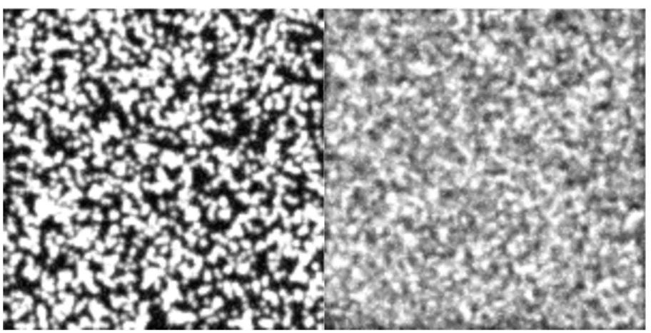
previously mentioned. Frames from a sample simulated data set are shown in figure 1.

iMSD analysis

Analysis via image mean square displacement (iMSD) was conducted on samples

to cross verify the diffusion values measured by STICS and those predicted utilizing

Stokes-Einstein theory. Video Spot Tracker (CISMM at UNC-CH) was used to select

individual particles, which were then tracked to give frame-by-frame locations. The

resulting series of coordinates were used to generate mean square displacement (MSD)

vs. τ plots, and the slope of the fit in equation (6) was used to calculate the diffusion

coefficient, D.

MSD(τ)=4Dτ (Eq. 6)

In videos with high particle densities and/or noisy conditions, the tracking of particle

movement was conducted by hand using FIJI due to the inability of the Video Spot

Tracker program to accurately follow beads.

Computational utilization

Due to the computational resources required to generate simulated bead datasets

and run STICS, jobs were run on the BASS supercomputer at the University of North

Experimental bead datasets

Experimental datasets were created by suspending 20nm, 100nm, and 200nm

yellow-green carboxylic acid coated Invitrogen fluorospheres in sucrose solutions.

Aliquots of the suspensions were then imaged using a 40x oil objective in a microscope

chamber held at 37°C. Frames from a sample experimental bead dataset are shown in

figure 2.

III. RESULTS

Findings from simulated datasets Verification of simulation using iMSD

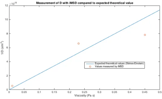
Image MSD analysis was conducted on simulated datasets to ensure the

simulation would provide sample videos with diffusion coefficient values aligning with

those predicted by Stokes-Einstein. This agreement is shown in figure 3, in which

diffusion values measured by iMSD for various datasets simulated over a range

viscosities agree with the predicted Stokes-Einstein values. The deviation from the

expected values is likely attributable to the small sample set of beads that could be

successfully tracked.

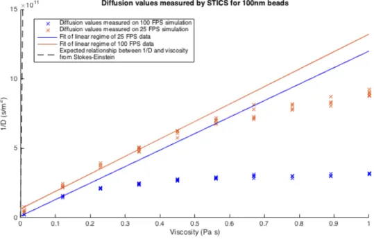
Ability of STICS to measure linear relationship between 1/D and viscosity For initial STICS validation 100nm particles were simulated at varying

viscosities, and the resulting videos were analyzed at 100 frames per second (FPS) using

STICS. A plot of 1/D versus viscosity in figure 4 shows a linear regime, where an

increase in viscosity corresponds to the expected linear increase in 1/D (the regions fitted

in figure 4). The linear component is represented as a modified version of Stokes-Einstein

(Eq. 7)

1

D= β⋅

6πr kBT

⎛

⎝

⎜ ⎞

where represents viscosity, r represents particle radii, T represents temperature, kB

represents the Boltzmann constant, and represents a calibration factor. For the linear

region of the 100 FPS simulations in figure 4 we calculate β=0.0055 _{with a correlation}

score of 0.95. As shown in figure 4, we note that this linear regimen is extended when the

frame rate of the simulation is decreased from 100 FPS to 25 FPS with βchanging

minimally, 5%, to β=0.0052with a correlation score of 0.99.

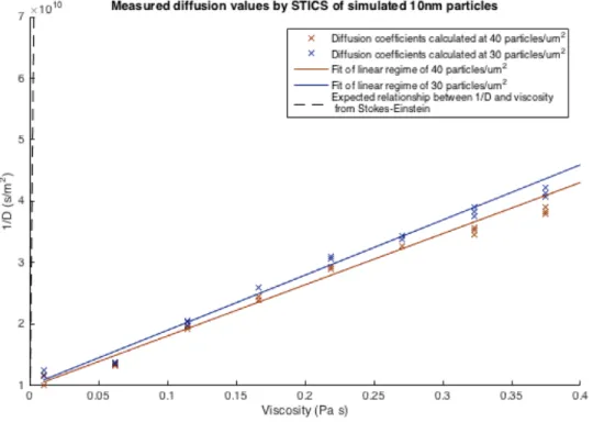
Effect of changing particle density

We then wished to elucidate which parameters influence β, beginning with

particle density. We decided to determine the impact of varying particle density by

simulating 10nm particles at 30 particles/um2 and 40 particles/um2 across varying

viscosities, the results of which are displayed in figure 5. Again we noticed a linear

region, in this case up to η<0.4Pa⋅s, and fit the data to equation 7. We see that the value

of β changes with particle density from β=0.0031(r = 0.91) with 30 particles/um2 to

β=0.0039(r = 0.96) with 40 particles/um2, representing a 25% increase in β for a 33%

increase in particle density.

Findings from experimental datasets

Differences between theoretical predictions and PIV measurements

Whereas in the simulated datasets iMSD showed agreement between visualized

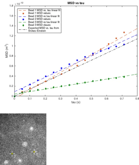
diffusion and that predicted by Stokes-Einstein, the same does not hold for experimental

bead videos. MSD plots for individual 100nm beads in a given video show varying

diffusion coefficients (figure 6), and even when averaged across multiple beads to

calculate average diffusion coefficients for the video we see differing values between the

iMSD calculated values and theoretical predictions (figure 7). These differences in

η

expected and observed diffusion coefficients could arise from imprecise temperature

control, bead clustering affecting effective particle radii, and errors in the viscosity

measurements of the standards, all of which contribute to the calculation of D using

Stokes-Einstien. Thus, due to the inability to calibrate STICS against values predicted by

Stokes-Einstein, we decided to correlate measurements from STICS with those measured

by iMSD.

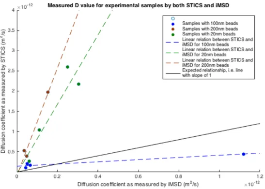
Linear relationship between diffusion coefficients measured by iMSD and STICS Given that we were unable to compare STICS measurements to theoretical values,

we compared D values measured by STICS to D values measured by iMSD to determine

if measurements in experimental datasets differed from expected values by a calibration

factorβ. Bead suspensions were prepared with 20nm, 100nm, and 200nm beads in H2O,

2M sucrose, and 2.5M sucrose solutions at 1% concentrations from the original bead

stock solutions. Each suspension was then analyzed using both iMSD and STICS. The

resulting values are graphed in figure 8, with the diffusion coefficient as measured by

iMSD on the x-axis and the diffusion coefficient measured by STICS on the y-axis.

Samples in which either iMSD was not possible due to an inability to effectively track

beads or which were too noisy for STICS are not depicted. The resulting plots show

linear relationships between DS, the diffusion coefficient value measured by STICS, and

D, the diffusion coefficient value measured by iMSD, for each set of beads. Specifically,

we observe D=βD_Swhere β=0.075, β=3.703, and β=0.117 with correlation coefficients

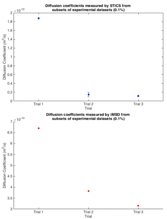
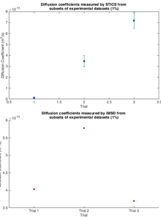
Consistency of STICS within subsamples

If the STICS measurements differ from expected values by a calibration factor β

that depends on the experimental setup, then measurements from subsamples of the same

setup should differ by the same β. To test this, videos of 200nm particles in 2M sucrose

at particle densities of 0.1% and 1% (sample frames shown in figure 2) were split into

multiple videos and individually analyzed using STICS. Each trial in figure 10 represents

one recording of beads diffusing in solution that was split into 3 separate movies, each of

which was then analyzed using STICS. The mean of the 3 movies for each trial is

presented in figure 10 along with their standard deviation. Image MSD analysis was also

done for each of the trials, and the resulting diffusion coefficients are plotted on figure 9

as well. Diffusion coefficients as measured by iMSD have a standard deviation of

1.38×10−14_m2_/sacross the 6 trials, whereas the standard deviation across trials as measured

by STICS is 7.02×10−13_m2_/s. In contrast, the mean standard deviation of D amongst

movies within a given trial as measured by STICS is only 3.23×10−14_m2_/s. This indicates

that the diffusion coefficient measured by STICS is consistent within a movie, but differs

from iMSD measured D’s by a different amount across movies. In other words, within a

given movie diffusion coefficients calculated by STICS appear to be off by a certain

calibration factor, β, from iMSD values, but this factor changes for different movies.

IV. DISCUSSION

The ability of STICS to measure diffusion shows promise, but is yet to be fully

validated. Its ability to measure a linear relationship between 1/D and η in simulated

datasets (figures 4 and 5) and the consistency with which it measures D values for

measure diffusion, but needs to be calibrated by a cofactor β that depends on the

experimental setup. This β takes the form of D=βDS where D is the actual diffusion

coefficient and DS is the value measured by STICS.

Through simulated datasets we have shown that when bead density and particle

size are kept constant, STICS is able to measure the expected linear relationship between

the viscosity of the solution, η, and the inverse diffusion coefficient, 1/D. The linear

region where this relationship holds necessitates sufficient movement of particles

between frames. As we see in figure 4, the linear region for the 100 FPS video extends

only to 0.1 Pa s, but when the video is down sampled to 25 FPS the linear region extends

to 0.4 Pa s. With smaller changes between frames the Gaussians evolve less for a given τ

value, and so the changes in peak width and location become harder to distinguish from

noise – hence the extension of the linear region when the video is down sampled. With

constant bead size and particle density, we see that β remains constant, hence the linear

relationship between 1/D and η. However, when certain conditional parameters change,

such as particle density,β also changes.

Because we are not able to trust the viscosities of the standards, in part due to

uncertainties in temperature, we decided to validate the STICS measurements against

those from iMSD. Furthermore, as shown in figure 6, MSD vs. τ plots of experimental

videos show individual beads have differing rates of diffusion, a possible result of beads

clumping in different amounts, especially at higher bead densities, and resulting in a

range of effective radii. In figure 9 we see that for a given experimental setup with

multiple videos taken of the same region, the measurements of D by STICS differ from

changes, possibly attributed to localized differences in particle density or other factors

that β could depend on.

The origin of the calibration factor, β, is yet to be determined – its

characterization and an understanding of its roots is the final hurdle in being able to

measure diffusion using STICS. A large issue with characterizing the calibration factor

lies in the creation of experimental standards with well-characterized parameters. These

parameters include viscosity, particle radii, and temperature of the suspension. In future

experiments the viscosity of standards with beads in suspension could be determined

more precisely using cone and plate viscosity measures. Using beads with alternative

coatings could reduce bead clumping and thus ensure constant particle radii. Lastly,

ensuring the suspension equilibrates to the set temperature of the chamber on the

microscope stage could control temperature. These parameters dictate diffusion rates, and

when they are controlled we would expect variation in D as measured by STICS to be

due to changes in β, not the actual diffusion rate. Parameters of interest to consider that

could affect β are particle density in the region being imaged, which we already believe

to play a role, signal strength, signal-bleaching rate, and imaging plane thickness.

A full characterization of β’s dependence on these parameters, and others it may

depend on, would allow us to essentially calibrate STICS for a given experimental setup.

That setup is not limited to beads diffusing in a suspension, but could easily be extended

to observing intranuclear molecular flow and diffusion without the constraints of current

measurement techniques, opening a novel door to study the physical landscape inside the

V. Figures

Figure 1. (Left) Sample frame from simulated bead dataset with 100nm beads. (Right) Sample frame from simulated bead dataset with 10nm beads.

Figure 2. (Left) Sample frame from experimental bead dataset with 200nm beads at a 1% concentration. (Right) Sample frame from experimental bead dataset with 200nm beads

Figure 3. Inverse of diffusion values measured by iMSD (red circles) for simulated datasets generally agrees with the linear prediction of Stokes-Einstein (blue line).

Deviation observed from expected values is likely due to small sample size of beads that

Figure 4. Measurement of 1/D by STICS for simulated 100nm bead datasets shows an expected linear region in both the 100 FPS and 25 FPS simulations with only a 5%

difference in their slope, but the linear region extends from 0.1 Pa s for 100 FPS to 0.4

Pa s for 25 FPS. However, both linear relations differ in their slope from the expected

Figure 5. Measurement of 1/D by STICS for simulated 10nm particles shows a linear regime with respect to viscosity. Increasing the particle density in the simulation by 33%

from 30 particles/um2 to 40 particles/um2 increases the value of β by 25% from 0.0031

Figure 6. (Top) MSD vs. τplot for the 3 beads identified in the experimental setup

pictured in the bottom image. Varying rates of diffusion between the three beads could

imply bead clustering, increasing the effective radius and thus decreasing the diffusion

rate as seen in bead 3. (Bottom) Sample frame from experimental 100nm bead dataset in

Figure 7. The D values measured using iMSD across different parameters differ from the Stokes-Einstein theoretical predictions by varying amounts, potentially due to bead

Figure 8. Due to the inability to calibrate STICS against theoretical values predicted by Stokes-Einstein, we calibrate the STICS measured D (vertical axis) against the D value

measured by iMSD (horizontal axis). The resulting plot shows linear relationships for

each size of bead, with β=0.075, β=3.703, and β=0.117 for the 200nm, 100nm, and

Figure 9a. Three trials of experimental bead dataset videos (200nm beads in 2M sucrose at a 0.1% bead density) were subsampled and analyzed with STICS. The mean D of the

subsamples and their standard deviation for a given trial is plotted on the graphs, as is the

Figure 9b. Three trials of experimental bead dataset videos (200nm beads in 2M sucrose at a 1% bead density) were subsampled and analyzed with STICS. The mean D of the

subsamples and their standard deviation for a given trial is plotted on the graphs, as is the

VI. REFERENCES

1. Alenghat, F., Ingber, D. (2002). Mechanotransduction: all signals point to cytoskeleton, matrix, and integrins. Science, 119.

2. Amira, B. B., Driss, Z., & Abid, M. S. (2015). Experimental study of the up-pitching blade effect with a PIV application. Ocean Engineering, 102, 95-104.

3. Dado, D., Sagi, M., Levenberg, S., & Zemel, A. (2012). Mechanical control of stem cell differentiation. Regenerative medicine, 7(1), 101-116.

4. Gavara, N., & Chadwick, R. S. (2012). Determination of the elastic moduli of thin samples and adherent cells using conical atomic force microscope tips. Nature nanotechnology, 7(11), 733-736.

5. Hedde, P. N., Stakic, M., & Gratton, E. (2014). Rapid measurement of molecular transport and interaction inside living cells using single plane illumination.

Scientific reports, 4.

6. Hebert, B., Costantino, S., Wiseman, P. (2005). Spatiotemporal image correlation spectroscopy (STICS) theory, verification, and application to protein velocity mapping in living CHO cells. Biophysical Journal, 88, 3601-3614.

7. Holenberg, Y., Lavrenteva, O. M., Liberzon, A., Shavit, U., & Nir, A. (2013). PTV and PIV study of the motion of viscous drops in yield stress material.

Journal of Non-Newtonian Fluid Mechanics, 193, 129-143.

8. Kuimova, M. K., Botchway, S. W., Parker, A. W., Balaz, M., Collins, H. A., Anderson, H. L., ... & Ogilby, P. R. (2009). Imaging intracellular viscosity of a single cell during photoinduced cell death. Nature Chemistry, 1(1), 69-73. 9. Li, G., & Reinberg, D. (2011). Chromatin higher-order structures and gene

regulation. Current opinion in genetics & development, 21(2), 175-186.

10.Lodish H, Berk A, Zipursky SL, et al. Molecular Cell Biology. 4th edition. New York: W. H. Freeman; 2000. Section 20.1, Overview of Extracellular Signaling. Available from: http://www.ncbi.nlm.nih.gov/books/NBK21517/

11. O’Donoghue, M. B., Shi, X., Fang, X., & Tan, W. (2012). Single-molecule

atomic force microscopy on live cells compares aptamer and antibody rupture forces. Analytical and bioanalytical chemistry, 402(10), 3205-3209.

12.Raman, A., Trigueros, S., Cartagena, A., Stevenson, A. P. Z., Susilo, M.,

Nauman, E., & Contera, S. A. (2011). Mapping nanomechanical properties of live cells using multi-harmonic atomic force microscopy. Nature nanotechnology, 6(12), 809-814.

13. Ribeiro, A. J., Denisin, A. K., Wilson, R. E., & Pruitt, B. L. (2015). For whom the

cells pull: Hydrogel and micropost devices for measuring traction forces.

Methods.

14.Schwarz, U. S., & Gardel, M. L. (2012). United we stand–integrating the actin cytoskeleton and cell–matrix adhesions in cellular mechanotransduction. Journal of cell science, 125(13), 3051-3060.

15. Wirtz, D., Konstantopoulos, K., & Searson, P. C. (2011). The physics of cancer:

VII. ACKNOWLEDGEMENTS

I would like to thank my mentor for this project, Dr. Michael Falvo, without whom

this work would not have been possible. I would also like to extend thanks to Dr. Richard

Superfine and the rest of the NSRG lab group for their support and feedback throughout

the project, with special thanks to Dr. Timothy O’Brien, Kellie Beicker, and Jeremy

Cribb. Lastly I would like to thank Dr. William Kier for his guidance and the BIOL692H