Reports on Progress in Physics
N Q Hung et al
Pairing in excited nuclei: a review
Printed in the UK 056301 RPPHAG
© 2019 IOP Publishing Ltd 82
Rep. Prog. Phys.
ROP
10.1088/1361-6633/ab05ac
5
Reports on Progress in Physics
Contents
1. Introduction ...2
2. Pairing within the uniform model ...4
2.1. BCS Hamiltonian within the grand canonical ensemble at fixed angular momentum ...4
2.1.1. General theory. ...4
2.1.2. Level density and statistical quantities. ...5
2.2. Applications of the theory to the uniform
model ...6
2.2.1. Single-particle model. ...6
2.2.2. Dependence of gap parameter upon angular momentum at zero temperature
(β =∞). ...6
2.2.3. Dependence of gap parameter upon angular momentum and excitation energy. ...6
2.2.4. Transition from temperature scale to energy scale. ...8
2.2.5. Entropy. ...9
2.2.6. Level-density denominator...9
2.3. Completeness of formalism with respect to angular momentum ...9
Pairing in excited nuclei: a review
N Quang Hung1 , N Dinh Dang2 and L G Moretto3
1 Institute of Fundamental and Applied Sciences, Duy Tan University, Ho Chi Minh city 700000, Vietnam 2 Quantum Hadron Physics Laboratory, RIKEN Nishina Center for Aceelerator-Based Science,
2-1 Hirosawa, Wako City, 351-0198 Saitama, Japan
3 University of California, Berkeley and Lawrence Berkeley National Laboratory, 1 Cyclotron Road, Berkeley, CA 94720, United States of America
E-mail: [email protected], [email protected] and [email protected]
Received 26 July 2017, revised 21 November 2018 Accepted for publication 8 February 2019 Published 17 April 2019
Corresponding Editor Professor Gordon Baym
Abstract
The present review summarizes the recent studies on the thermodynamic properties of pairing in many-body systems including superconductors, metallic nanosized clusters and/or grains, solid-state materials, focusing on the excited nuclei, that is nuclei at finite temperature and/ or angular momentum formed via heavy-ion fusion, α-induced fusion reactions, or inelastic scattering of light particles on heavy targets. Because of the finiteness of the systems, several interesting effects of pairing such as nonvanishing pairing gap, smoothing of superfluid-normal phase transition, first and second order phase transitions, pairing reentrance, etc, will be discussed in detail. Influences of exact and approximate thermal pairing on some nuclear properties such as temperature-dependent width of the giant dipole resonance, total level density, and radiative strength function of the γ-rays emission will be also analyzed. Finally, the first experimental evidence of the pairing reentrance phenomenon in a 104Pd nucleus
as well as its solid-state counterpart of ferromagnets under strong magnetic field will be presented.
Keywords: pairing correlation, excited nuclei, hot rotating nuclei, phase transition, statistical nuclear thermodynamics, giant dipole resonance, nuclear level density and radiative strength function
(Some figures may appear in colour only in the online journal)
Review
IOP
2019
1361-6633
https://doi.org/10.1088/1361-6633/ab05ac
2.4. Effect of single-particle spin projection
distribution upon the shape of the yrast line ...9
2.5. Transition from the constant spacing model to the shell model ...10
2.6. Thermodynamic properties of paired nucleus with fixed number of quasiparticles ...11
2.6.1. Hamiltonian. ...11
2.6.2. Grand partition function and other thermodynamic quantities. ...11
2.6.3. Limiting properties for T = 0 (β → ∞). ...12
2.6.4. Properties of the system for T > 0. ...13
2.7. Experimental level densities and first-order pairing phase transition ...15
3. Grand-canonical ensemble treatment of pairing problem within the Hartree–Fock–Bogoliubov theory and finite-temperature pairing reentrance ...16
3.1. Hartree–Fock–Bogoliubov theory for hot and hot rotating nuclei ...16
3.2. Finite-temperature pairing reentrance in even–even nuclei ...20
3.3. Finite-temperature pairing reentrance in odd nuclei ...21
4. Canonical and microcanonial treatments of pairing problem ...23
4.1. Particle-number projection ...23
4.2. BCS with Lipkin–Nogami particle number projection plus self-consistent quasiparticle random-phase approximation incorporated into the canonical and microcanonical ensembles ...25
4.3. Exact solutions within the canonical and microcanonical ensembles ...28
4.4. Shell model Monte Carlo method at finite temperature ...30
5. Experimental evidences ...32
5.1. Experimental evidence of pairing reentrance in nuclei ...32
5.2. Condensed-matter counterpart: magnetic-field-induced superconductivity ...34
5.2.1. Magnetic-field-induced superconductivity based on Jaccarino–Peter compensation effect. ...35
5.2.2. Unconventional magnetic-field-induced superconductivity: Reentrant superconductivity. ...36
6. Role of pairing in properties of excited nuclei ...37
6.1. Effect of thermal pairing on giant dipole resonance in hot nuclei ...37
6.1.1. Effect of BCS pairing on energy and line shape. ...37
6.1.2. Effect of modified BCS and exact pairing on the width of giant dipole resonance within phonon-damping model. ...38
6.1.3. Effect of pairing fluctuation on the width of giant dipole resonance within thermal shape fluctuation model. ...39
6.2. Effect of exact thermal pairing on nuclear level density and radiative strength function...41
7. Summary and outlook ...43
Acknowledgments ...44
References ...44
1. Introduction
Pairing correlation is a common feature characterizing the superconducting (superfluid) properties of strongly interact-ing many-body systems ranginteract-ing from the very large ones such as neutron stars to the tiny ones such as atomic nuclei. In macroscopic and/or infinite systems such as low-temperature superconductors, pairing correlation decreases with increas-ing temperature T or excitation energy and completely van-ishes when the temperature reaches a critical value T=Tc,
called critical temperature. As the result, the system under-goes a phase transition from superfluid to normal phases (superfluid-normal phase transition). This phenomenon was explained very well by the Bardeen–Cooper–Schrieffer (BCS) theory of superconductivity [1]. The latter was pro-posed based on an assumption that two electrons, one with spin up and one with spin down, in superconductors tend to couple to form a so-called Cooper pair at low temperatures. The condensation of a set of Cooper pairs is responsible for the superconductivity of the materials. Pairing has been found to have a significant contribution in the study of vari-ous systems including liquid helium [2], neutron stars [3–5], interacting spins [6, 7], metal clusters [8–10], quantum dots [11], ultrasmall metallic grains [12, 13], etc. The BCS theory predicts the value of the critical temperature Tc, at which the
pairing gap collapses, to be Tc≈0.568∆(0), where ∆(0) is
the pairing gap at zero temper ature. After the introduction of the BCS, Bohr, Mottelson, and Pines recognized the similar-ity between the electron pairs in superconducting materials and the nucleon (neutron or proton) pairs observed in atomic nuclei [14, 15] and proposed the nuclear superconductivity (superfluidity). Applications of the BCS theory to nuclear system, explicitly performed by Belyaev [16, 17], Soloviev [18, 19], and others [20–29] showed that pairing correlation affects most of the nuclear structure properties, from binding energy, single-particle orbitals to excitation spectra, transition probabilities, collective vibrational and rotational excitations, deformation, thermal properties, level density, etc. In excited nuclei, the increase of temperature or excitation energy breaks the nucleon pairs located around the Fermi levels, which are responsible mostly for the pairing correlation. The unpaired nucleons scatter to the single-particle levels nearby, entirely block them because of the Pauli exclusion principle. This causes the decrease of pairing correlation. When temper ature is high enough, reaching its critical value Tc, all the nucleon
rotating nuclei vanishes after all the nucleon pairs are broken. This is the well-known Mottelson–Valatin effect [20].
However, when both temperature and angular-momentum effects act together as in hot rotating nuclei, there appears an anomalous phenomenon, called pairing reentrance. This phenom enon, which was first introduced by Kamuri [23], occurs when the angular momentum of the nucleus is slightly higher than its critical value Jc. When it takes place, the
pair-ing correlation, which is zero at low temperature, becomes nonzero at a certain temperature, and increases to reach a maximum, then decreases to vanish at a higher temperature. This phenomenon was later confirmed by Moretto [25, 26] by extending the BCS theory to finite temperature and angu-lar momentum and applied it to the nuclear uniform model. The recent study of the projected pairing gaps in ultra-small metallic grains for even and odd numbers of particles also found such anomalous pairing or pairing reentrance (see e.g. figure 9 of [30]). A similar effect called unconventional super-conductivity has been recently discovered in the experimental study of superconducting URhGe material in the present of magnetic field H [31], whose role is similar to the rotation in nuclei. In this experiment, the URhGe material in the normal state at the applied magnetic field around 2 T becomes super-conducting at low temperature as the magnetic field increases up to the values between 8 and 13 T.
Indeed, all the above predictions of the pairing reentrance phenomenon are the results of using the BCS theory. This the-ory is precise only in infinite and/or very large systems, where the average size of the Cooper pairs (coherence length) is nor-mally large and thermal fluctuations are negligible. For small systems such as underdoped cuprates, where the coherence length is very short, the thermal fluctuations are no longer small, which require a serious reexamination of the BCS the-ory [32]. Similarly, nuclear system is expected to have large thermal fluctuations due to its finiteness (small number of nucleons compressed into a fixed volume with the diameter of several fermi). Various theoretical studies of the effect of ther-mal fluctuations on pairing in atomic nuclei have been under-taken in the past three decades. In the pioneering works by Moretto [24], who employed the macroscopic Landau theory of phase transition to evaluate the most probable value of the pairing gap in a uniform model of nuclear pairing problem, it has been pointed out that the average pairing gap does not collapse at the critical temperature as predicted by the BCS theory but monotonically decreases with increasing temper-ature. Consequently, the superfluid-normal phase trans ition observed via the discontinuity of the associated specific heat is smoothed out. This approach was later employed by Goodman [33, 34] to include the thermal fluctuations in the Hartree–Fock–Bogoliubov (HFB) theory at finite temper-ature. The calculations within the static-path approximation (SPA), in which thermal fluctuations are taken into account by taking the thermal average over all static paths around the mean field, also came to the non-vanishing of pairing gap at finite temperature, in agreement with the predictions by Moretto and Goodman in [25, 33]. This result was later reconfirmed by the shell model [35] and shell-model Monte Carlo [36] calculations for realistic nuclei. Recently, by taking
into account the effect of quasiparticle-number fluctuations in the BCS pairing, two microscopic approaches, called modi-fied BCS (MBCS) [37] and finite-temperature BCS1 [38] theories, have been proposed, which pointed out that the quasiparticle-number fluctuations are indeed the microscopic origin that causes the non-vanishing of thermal pairing gap in finite small systems. The predictions of the above-mentioned approaches are in qualitative agreement with the empirical pairing gap of 184W nucleus extracted from the experimental
nuclear level densities [39] as well as that obtained by incor-porating the exact solutions of the pairing Hamiltonian into the canonical and grand canonical ensembles [40]. The effect of non-vanishing thermal pairing has also been included in the phonon damping model (PDM) for describing the width of the isovector giant dipole resonance (GDR). The results obtained show that, because of non-vanishing thermal pairing, the GDR width remains almost unchanged, or even reduced at the temper ature T 1 MeV, in good agreement with the exper-imental data [37, 41–43]. It is worthwhile to mention that this nearly temperature-independent value of the experimental GDR width at low temperature was not previously explained in other approaches, which either include only the BCS pair-ing or neglect pairpair-ing. A similar conclusion on the temperature dependence of the GDR width has been made by including thermal pairing fluctuations in the thermal shape fluctuation model, which cause the noncollapsing average pairing gaps [44]. Moreover, a very recent unified microscopic approach based on the exact solutions of the pairing Hamiltonian at zero temperature has been proposed. These exact solutions are incorporated into the canonical ensemble and then com-bined with the finite-temperature independent-particle model as well as the PDM to simultaneously describe, for the first time, two key quantities of hot nuclei, namely nuclear level density and radiative strength function of the γ-ray emission, which are important for the description of low-energy nuclear reactions as well as nucleonsynthesis in stars [45]. It has been shown in [45] that exact thermal pairing, which results in the non-vanishing of pairing gap and smoothing of the superfluid-normal phase transition, plays an important role in the descrip-tion of the total nuclear level density as well as the radiative strength function of excited nuclei in the energy region below the particle-separation energy.
solvable shell-model Hamiltonian at finite temper ature and total angular momentum [47] showed a similar pairing reen-trance effect. This behavior of pairing reenreen-trance was also reconfirmed by the calculation within the BCS1 approach at finite temperature and angular momentum [48]. From the theor etical points of view, the pairing reentrance in atomic nuclei can be predicted via the behavior of calculated pairing gaps. However, from the experimental side, it is not simple, if not at all feasible, to extract the thermal pairing gap because of the admixture of uncorrelated single-particle configurations, which should be properly excluded from the extension of the formula for the odd–even mass difference [40].
Meanwhile, the heat capacity can be extracted from the experimental level densities by interpolating the level density data up to a very high excitation energy of about 100 MeV using the phenomenological back-shifted Fermi gas formula [49–51]. Consequently, the existence of a bump or an S-shape on the curve of the heat capacity around the critical temper-ature was observed, which allows us to discuss the smoothing of the transition from the superfluid phase to the normal one in hot nuclei. The recent calculation within the shell-model Monte-Carlo method (SMMC) for the heat capacity of a heated rotating 72Ge nucleus has shown that there appears a
local dip in the heat capacity at a rotational frequency of 0.5 MeV and temperature T∼0.45 MeV, and a local maximum on the temperature dependence of the logarithm of level den-sity is observed at the same rotational frequency and temper-ature [52]. These irregularities in the heat capacity and level density are associated with the signatures of the pairing reen-trance. The results obtained within the BCS1 at finite temper-ature and angular momentum for the same 72Ge nucleus [53]
agree with the SMMC prediction for the local minimum in heat capacity, however, no pronounced local maximum in the temperature-dependent level density is seen in this calculation. At the same time, pairing reentrance is seen in the proton pair-ing gap in [53], whereas this effect is claimed in the neutron pairing energy in [52]. This difference might occur because of using the same single-particle spectra for both protons and neutrons in [52], that is, neglecting the Coulomb interaction in the SMMC calculation, as has been pointed out in [53]. The detection of pairing reentrance phenomenon is therefore still under question. Very recently, in a series of experiments car-ried out for the reaction 12C + 93Nb →105Ag∗→104Pd* + p at the incident energy of 40–50 MeV [54–58], an enhance-ment of level density has been observed in 104Pd nucleus at
low excitation energy (temperature) and high angular momen-tum, which is quantitatively similar to that reported in [52]. Immediately after that, the analysis of the BCS1 at finite temper ature and angular momentum was carried out for the same warm rotating 104Pd nucleus and the results obtained for
the level density agree quite well with the observed data, indi-cating the first evidence of pairing reentrance phenomenon in this nucleus [59, 60].
The present review summarizes the recent studies on the pairing properties in finite systems, focusing on excited nuclei, that is at finite temperature and/or angular momentum. The review is organized as follows. Section 2 introduces the
pairing properties based on the BCS Hamiltonian within a simple uniform model. The phase diagram boundaries of the paired regions with the associated phase transitions such as the first-order and second-order ones in the cases with fixed total angular momentum, fixed quasiparticle number, and fixed energy will be discussed in detail. The treatments of nuclear pairing problem within the grand canonical, canoni-cal, and microcanonical ensembles by using several theor-etical approaches will be discussed in sections 3 and 4. Section 5 presents the exper imental evidences of the pairing reentrance in hot rotating nuclei and solid-state counter part under a strong magnetic field. The role of pairing in the prop-erties of excited nuclei such as giant dipole resonance, total nuclear level density, and radiative strength function will be highlighted in section 6. The review is summarized in the last section, where conclusions are drawn and an outlook is given.
2. Pairing within the uniform model
2.1. BCS Hamiltonian within the grand canonical ensemble at fixed angular momentum
2.1.1. General theory. We shall calculate all the statisti-cal nuclear properties using an arbitrary shell-model level sequence, including pairing and angular momentum within a generalized BCS Hamiltonian. The standard procedure usu-ally consists of restricting the grand partition function of the system with the constraints to conserve energy, number of particles, and, in general, any other first integral of motion. However, only the first integrals that are expansible in terms of sums over single-particle states can be easily handled in this way. Regarding the total angular momentum, only its z-projec-tion M has this property. Therefore the following calculaz-projec-tions are restricted to a constant angular momentum z-projection M. Such a procedure is justified and the formalism is complete in most of cases as will be shown in this section.
The pairing Hamiltonian H of a Fermi gas with an attrac-tive and constant pairing interaction has the following form in the second quantization [14]
H=
±k
ka†kak−G
kk a†
−ka†kaka−k,
(1)
where k are the single-particle energies; a†k and ak are the particle creation and annihilation operators; and G is the pair-ing strength. Here, for simplicity, the subscripts k denote the single-particle states |k,mk in the deformed basis with posi-tive single-particle spin projection mk, whereas those with −k stand for the time-reversal states |k,−mk. Including the straints on particle number and angular momentum, it is con-venient to consider a modified Hamiltonian in the form [25]
H→H−λN−γM,
(2) where N is the particle number, M is the projection of the total angular momentum on a laboratory-fixed z-axis or on a body-fixed z-axis, and λ and γ are two Lagrange multipliers
N= ±k
a†
kak, M=
k
mka†kak− −k
mka†−ka−k. (3)
The Hamiltonian, modified as in (2), is then rewritten as
H=
k
ζk+a†kak+ −k
ζ−−ka†−ka−k
−G
kk a†
−ka†kaka−k, (4)
where ζk+=k−λ−γmk and ζk−=k−λ+γmk. Such Hamiltonian can be approximately diagonalized by means of the Bogoliubov transformation [61, 62]
a†
k =ukα†k+vkα−k, a−k=ukα−k−vkα†k, (5) where α†k and α−k are the quasiparticle creation and destruc-tion operators, respectively, whereas uk and vk are the Bogoliubov’s coefficients satisfying the normalization condi-tion u2
k+v2k=1.
By substituting (5) in (4) and retaining only the diagonal terms, one obtains
H=v2k(ζk++ζk−) +
n+
k(ζk+u2k+ζk−v2k)
+n−k(ζk−uk2+ζk+v2k)−G kk
ukvk(1−n+k −n−k)
2 ,
(6) where n±
k =ᆱkα±k are the quasiparticle occupation num-bers. Minimizing (6) with respect to uk and keeping n+k and n−k constant, one obtains the Hamiltonian
H=(k−λ−Ek) +
n+
k(Ek−γmk)
+n−k(Ek+γmk) +∆
2
G , (7)
and the gap equation
2
G=
1−n+
k −n−k
Ek ,
(8)
with Ek=
(k−λ−Gv2k)2+ ∆2 being the quasiparticle energies [25].
The grand partition function Ω can be directly obtained from the Hamiltonian (2) by using the relation eΩ=Tre−βH. It is now given as
Ω =−β(k−λ−Ek)
+ln{1+exp[−β(Ek−γmk)]}
+ln{1+exp[−β(Ek+γmk)]} −β∆
2
G . (9)
The gap equation, which relates the quantities ∆, β, and γ,
takes now the form
f(∆,β,λ,γ) = 1 2Ek
tanh1
2β(Ek−γmk)
+tanh1
2β(Ek+γmk)
= 2
G. (10)
2.1.2. Level density and statistical quantities. The level den-sity is defined as the inverse Laplace transform of the grand partition function [26]
ρ(E,N,M) = 1 2πi
3 dβ
dα
dµeS,
(11)
where
α=βλ, µ=βγ, S= Ω−αN−µM+βE.
(12) This integral can be evaluated with good approximation at the saddle point of the exponent S, which is located at
N= ∂Ω
∂α, M= ∂Ω
∂µ, E=− ∂Ω ∂β.
(13)
This leads to the level density in the form
ρ(E,N,M) = e S
(2π)32D12,
(14) where D=
∂2Ω
∂α2 ∂
2Ω
∂α∂µ ∂2Ω ∂α∂β ∂2Ω
∂µ∂α ∂2Ω
∂µ2 ∂
2Ω
∂µ∂β ∂2Ω
∂β∂α ∂2Ω ∂β∂µ
∂2Ω ∂β2 , (15)
with both S and D to be evaluated at the saddle point. From the saddle-point conditions (13), the first integrals of the system can be explicitly calculated
N=
1−k−λ 2Ek
tanh1
2β(Ek−γmk)
+tanh1
2β(Ek+γmk)
, (16)
M=mk
1
1+exp[β(Ek−γmk)]
−1+exp[β(E1
k+γmk)]
, (17)
E=k
1−k−λ 2Ek
tanh1
2β(Ek−γmk)
+tanh1
2β(Ek+γmk)
−∆G2, (18)
S=
ln{1+exp[−β(Ek−γmk)]}
+ln{1+exp[−β(Ek+γmk)]}
+β Ek−γmk
1+exp[β(Ek−γmk)]
+β Ek+γmk
1+exp[β(Ek+γmk)]
The explicit form of second derivatives of Ω in (15) is given, e.g. in [26].
2.2. Applications of the theory to the uniform model
2.2.1. Single-particle model. The model consists of equi-distant doubly degenerate single-particle levels (Nilsson-like levels) with density g and constant angular momentum pro-jection mk = m. The levels are symmetrically located from both side of the chemical potential λ, which is set to zero at all temper atures (in general, within a non-symmetric model the chemical potential λ varies with the temperature). In the calcul ations discussed below when one is dealing with energy as a variable, the uniform model has been employed with the following parameters: g = 7 MeV−1, ∆
0=1.0 MeV, and m=2 to mimic a heavy rare-earth nucleus (∆0 is the gap
parameter at T = 0 and M = 0).
2.2.2. Dependence of gap parameter upon angular momen-tum at zero temperature (β=∞). Assuming the pairing correlation extending over an energy interval ±ω above and
below the Fermi surface and transforming all the summations over the single-particle levels into integrals within the limits ±ω, one obtains from (10) the gap parameter at T = 0 and
M = 0 as
∆ (20)0= sinh(ω1/gG) ≈2ωexp(−1/gG), (gG1).
The dependence of ∆ upon M for T = 0 is obtained by inte-grating (17)
∆ = ∆0(1−M/Mc)1/2,
(21) where
Mc=gm∆0,
(22) from which one immediately derives
d∆ dM
M=0
=− 1
2gm, Mlim→Mc = d∆
dM =−∞.
(23)
The dependence of ∆ upon M in (21) is plotted in figure 1, which shows that the gap parameter, i.e. the pairing correla-tion, decreases with increasing M to vanish at a critical value
Mc, determined by (22). Equation (23) expresses the slopes
of ∆ = ∆(M) for M = 0 and M = Mc. The qualitative
mean-ing of such results can be easily understood by considermean-ing the Hamiltonian (1), whose second term shows that, when-ever a pair of particles is transferred from a filled level to an empty one, there is an energy gain G. The first term, of course, means that, in order to transfer a pair of particles from a level k to a level k, one has to invest an amount of energy equal
to 2(k−k). In other words, the pairing interaction affects most the levels close to the Fermi surface. To generate angular momentum, one must break some of the pairs: the excitations arising in this way (quasiparticles) occupy the single-particle levels, which become unavailable (blocked) to the scattered pairs. Consequently, the pairing correlation decreases. When the angular momentum is sufficiently large, all the levels
around the Fermi one are blocked by quasiparticles, making the pairing correlation energetically unfavorable (figure 2).
2.2.3. Dependence of gap parameter upon angular momen-tum and excitation energy. In the absence of angular momen-tum (M = 0), the gap equation (10) gives the depend ence of ∆ upon T alone, which is shown in figure 3. The pair-ing correlation decreases with increaspair-ing T up to a critical temper ature Tc, where ∆ =0 and the pairing correlation
dis-appears altogether. The value of Tc is given by the relation
∆
/
∆0
0 0.2 0.4 0.6 0.8 1
M/Mc
0 0.2 0.4 0.6 0.8 1
T=0
Figure 1. Dependence of the gap parameter ∆ upon the angular momentum M at zero temperature. ∆0 is the gap parameter for
T = 0, M = 0 and Mc is the critical angular momentum above
which ∆ =0. Adapted with permission from [26], Copyright (1972) by Elsevier.
Tc=1.14exp(−1/gG), which consequently leads to the
well-known relation [63]
2∆0
Tc =3.53.
(24)
Again the decrease of the pairing correlation with T (excita-tion energy) is caused by breaking particle pairs, which gener-ate the quasiparticles, blocking the single-particle levels close to the Fermi surface. The combined effect of T and M can be seen by determining the dependence of the critical temperature upon the angular momentum projection M. Such a function defining the boundaries between the superfluid and the normal phase in the (M,T) plane is shown in figure 4. At 0M <Mc
the gap equation (10) yields a single solution for the critical temperature, which decreases with increasing M as expected. However, at MMc , the gap equation produces two critical
temperatures: the upper one is the continuation of the curve obtained at M < Mc, while the lower one starts from zero at M=Mc and coalesces with the upper one at M=1.22Mc.
Surprisingly for M>Mc, the system is in the normal phase
within the temperature range between zero and the lower criti-cal temperature, whereas it is in the superfluid phase within the temperature range between the lower and the upper critical temperatures. Above the upper critical temperature, the system returns to its normal phase again. We are dealing here with an unexpected effect, namely for M>Mc, a system in the
normal phase can become a superconductor by increasing its temperature or excitation energy. This is in dramatic contrast with the known case for M = 0 (figure 3), where an increase in temperature destroys the pairing correlation. We call this effect ‘anomalous pairing’ or ‘thermally assisted pairing correlation’ because it is sustained by increasing temperature.
A qualitative insight into such a peculiar phenomenon can be gained as follows. As stated previously, the angular
momentum, generated by breaking pairs of particles, puts the quasiparticles into the single-particle levels close to the Fermi surface and polarizes their spins. At T = 0, a sufficiently high angular momentum causes a large number of quasiparticles completely occupying the closest levels around the Fermi sur-face. Such a complete blocking of single-particle levels makes the pairing correlation energetically unfavorable (figure 5(a)). Increasing temperature tends to relax the tight packing of quasi particles by spreading them farther and farther away from the Fermi surface. Consequently, some single-particle levels become partially unoccupied and, therefore, become available
∆
/
∆0
0 0.2 0.4 0.6 0.8 1
T/Tc
0 0.2 0.4 0.6 0.8 1
M=0
Figure 3. Dependence of the gap parameters ∆ upon the temperature T at zero angular momentum. Tc is the critical
temperature above which ∆ =0. Adapted with permission from [26], Copyright (1972) by Elsevier.
T
(M
eV
)
0 0.2 0.4 0.6
M ( h )
0 2 4 6 8 10 12 14 16 18
Figure 4. Dependence of the critical temperature upon angular momentum. The parameters are the same as in figure 3. Adapted with permission from [26], Copyright (1972) by Elsevier.
again for pairs scattered by the pairing interaction (figure 5(b)). At a temperature equal to the lower critical temper ature, such a spreading out of quasiparticles is just sufficient to make the pairing correlation energetically favorable. A further increase of the temperature will increase the pairing correlation first but eventually produce the usual pairing breakdown by generating an increasingly large number of quasiparticles.
Such a remarkable effect persists also for values of M smaller than Mc, as can be clearly shown by calculating the
dependence of the gap parameter ∆ upon temperature and
angular momentum projection. To do so, we solve the set of two equations (10) and (17). In figure 6, the (T,M) plane is again divided into two regions, paired (superfluid) and nor-mal. It appears that for a constant M value below Mc, the
gap ∆ increases with T, reaches a maximum, decreases, and
finally vanishes at the critical temperature. For M>Mc, the
gap parameter ∆ stays equal to zero from T = 0 up to the
lower critical temperature. In the paired region, ∆ increases,
goes through a maximum, decreases again, and vanishes at the upper critical temperature. Notice that ∆ goes through
a maximum with increasing T for any non-zero value of M. This initial increase in ∆ with increasing T can also be called
thermally assisted pairing correlation, but hardly can be called anomalous. The effect at M = 0 could be called anomalous because only in such a case ∆ decreases monotonically with
increasing temperature.
2.2.4. Transition from temperature scale to energy scale. The canonical ensemble has been used in statistical calcul ations for excited nuclei because of the development of more advanced algorithms. Thus, the calculations presented so far should be understood to hold at a fixed temperature. However, for the great majority of purposes, excited nuclei are considered with a fixed excitation energy rather than with a fixed temperature. There-fore, it is more common to speak of nuclei in terms of energy instead of temperature and use the microcanonical ensemble
instead of the canonical ensemble in statistical calculations for nuclear systems. Even within the canonical ensemble, where the temperature is fixed and energy is allowed to fluctuate, it is possible to calculate the average energy associated with such a temperature. The main effect of such approximation is that of introducing some smoothing of the statistical quantities with respect to energy. The energy of the system at T = 0 calcu-lated as a function of M is called the yrast line and it is usually defined in a somewhat different fashion (like the function giv-ing the highest angular momentum for a given energy or alter-natively giving the lowest possible energy for a given angular momentum). For the uniform model, one obtains
E−E0= 12g∆20MM c
2−2MM
c
forM<Mc,
(25)
E−E0=12g∆20+ M 2
4m2g forM>Mc,
(26)
where E0 is the ground-state energy, e.g. energy at T = 0
and M = 0. The yrast line is shown in figure 7 (lower line) together with the critical energy as a function of M (upper line). These two curves, which join smoothly at Mc, define
the region of superfluid phase. The dashed line, as the con-tinuation of the yrast line given by (26) for M values lower than Mc, represents the yrast line corresponding to an
uncor-related Fermi gas. Such a line intersects the axis, at M = 0, at an energy equal to 1
2g∆20, which represents the condensation
energy from the normal to the superfluid phase at M = 0 and T = 0. The difference between the dashed line and the lower line represents the T = 0 condensation energy as a function
T
(M
eV
)
0 0.2 0.4 0.6
) (h M
0 2 4 6 8 10 12 14 16
Figure 6. Contour map of the gap parameter as a function both of temperature and angular momentum. The spacing in ∆ between two successive lines is 0.05 MeV from ∆ =1.0 to ∆ =0.1 MeV. The outer line corresponds to ∆ =0. Adapted with permission from [26], Copyright (1972) by Elsevier.
E
(M
eV
)
0 2 4 6 8 10 12
M ( h )
0 2 4 6 8 10 12 14 16 18 20
of M. Such a condensation energy vanishes together with the pairing correlation at M=Mc.
As a final simple insight into the change from temper ature to energy scale, figure 8, corresponding to figure 6, shows the lines of equal ∆-value in the (E, M) plane. The superfluid region, where the inner lines are located, is bounded by the yrast and critical energy lines, as two outer lines.
2.2.5. Entropy. The pairing effects are also very relevant in the entropy expression. Shown in figure 9 is the entropy as a function of M at several temperatures T. In the absence of pairing and in particular for M and T above their critical values, the entropy, at fixed T does not depend upon M. This appears clearly in the right side of the figure, where the curves reduce to equally space straight lines parallel to the M-axis. Within the superfluid region, there is a general depression in the entropy values, the lager entropy the lower T. At the very low T, the entropy goes through a maximum.
2.2.6. Level-density denominator. As has already been observed for the pairing correlation at M = 0 [63], the denom-inator of the level density undergoes a discontinuity at Tc. In
particular, at M>Mc, where two discontinuities should exist
with respect to the two values of the critical temperatures, corresponding to exceedingly small excitation energies, the validity of the saddle-point approximation is doubtful.
2.3. Completeness of formalism with respect to angular momentum
In the present formalism, only the first integrals can be easily handled by summing over single-particle levels. The energy, the particle number, and the z-projection M of the total angular
momentum satisfy such a requirement, but not the total angu-lar momentum J. An obvious lack of completeness in such a calculation can be seen, e.g. in the dependence of ∆ on M at T = 0 (figure 6). As the choice of the z-axis is arbitrary, so is the M projection on such an axis. It is, therefore, unclear how the intrinsic properties of the system, like the pairing correla-tion, depend on the arbitrary choice of the z-axis. However, the formalism is essentially complete at least for a spherical (or quasi-spherical nucleus), where any axis can be taken as the symmetry one. It is quite obvious that, if the total momentum is not aligned with the z-axis, the present formalism accounts only for a part of the overall angular momentum effect. But, if the angular momentum is indeed aligned with the z-axis (and this can always be the case if a suitable choice of z-axis is made), then there is no angular momentum comp onent left out, which may affect the intrinsic properties of the system. It follows that we can substitute the angular momentum in place of M in all the expression concerning intrinsic properties of the system. Such is the case for the expression giving ∆ as a function of M and T, for the yrast line expression, for the energy expression and so on [64, 65].
2.4. Effect of single-particle spin projection distribution upon the shape of the yrast line
As has been discussed, the uniform model with a constant spin projection distribution predicts a decreasing angular velocity (rotational frequency) with increasing angular momentum in the paired region. Consequently, the yrast line, which presents a negative second derivative and the moment of inertia as a function of the squared angular velocity, undergoes a back-bending. These effects strongly depend on the spin projection
E
(M
eV
)
0 2 4 6 8 10
M ( h )
0 2 4 6 8 10 12 14 16 18
Figure 8. Same as in figure 7. The contour lines in the paired region correspond to the regions of equal ∆ from ∆ =1 MeV to ∆ =0 MeV in steps of 0.1 MeV. Adapted with permission from [26], Copyright (1972) by Elsevier.
En
tr
op
y
0 2 4 6 8 10 12 14 16 18 20 22 24
M ( h )
0 2 4 6 8 10 12 14 16 18 20
distribution, whose version p(m)dm =δ(m−m)dm is
not very realistic. In [66, 67], a rectangular distribution was employed as
p(m)dm=
g(dm/m
x), if 0 mmx,
0, ifmmx,
(27)
which quite well approximates the 2j + 1 projection of a j -shell, and therefore is expected to be more realistic for a spherical nucleus. Here, mx is the largest possible spin pro-jection. For this distribution, it is also possible to carry out the analytic integration of the angular momentum and the gap equations.
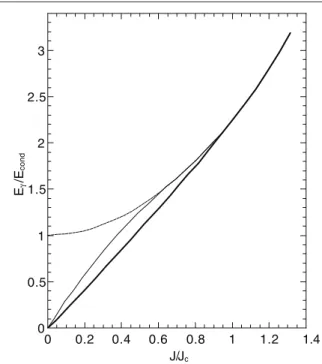
Shown in figure 10 is the complete function γ=γ(J), which monotonically increases with J, excluding the possi-bility of the back-bending with the critical angular momen-tum and the rigid moment of inertia given by Jc=13egmx∆0
and R= 23gm2x. The critical angular momentum predicted by the present model is larger that that given by the uniform model when the comparison at constant moment of inertia is made. The ratio R between the two critical angular momenta is R = (1/3)1/2e. The yrast line, which is now expected to have
a positive second derivative, can be calculated numerically. Its value at the critical angular momentum is
Eγ(J=Jc) = 12g∆20+ J 2 c 2R
=1
2g∆20(1+16e2)≈2.23Econd, (28)
where Econd =12g∆20 is the condensation energy owing to
pairing, in contrast with the uniform model, which predicts
Eγ(J=Jc) =1.5Econd (see e.g. equation (32) of [67]). The
complete yrast line, presented in figure 11, shows the expected small positive second derivative.
2.5. Transition from the constant spacing model to the shell model
While the uniform model brings forth the pairing features, this approximation may be oversimplified. Within this model, it has been shown how the yrast line changes dramatically by replacing the m distribution as a delta function picked at the average m with a rectangular distribution for 0mmx at the same average value. More dramatic changes take place when the equally spaced single-particle levels are substi-tuted with the shell model levels. Moving the Fermi surface from one degenerate level to another leads to the associated changes in the local single-particle level densities and spins, which dramatically affect the pairing correlation as a function of excitation energy and angular momentum.
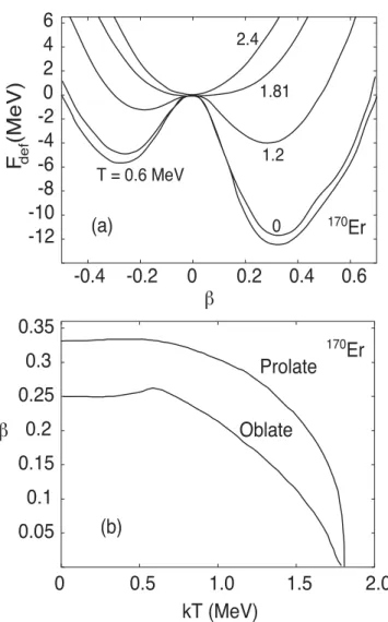
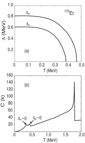
Shown in figure 12 are the gap parameters for neutrons and protons as a function of temperature and angular momentum for the nucleus 220Rn. The figure shows that both temperature
and angular momentum affect pairing, leading to a second-order phase transition line where the gap param eter vanishes. On the other hand, the thermally assisted pairing does not show up in the proton component and remains rather weak in the neutron one. In figure 13, the lines of constant entropy are shown in the (T,J) plane, where the difference between the proton and neutron components is more obvious. Here the second-order criticality line clearly shows a pairing reentrance for the neutron component but not for the proton one.
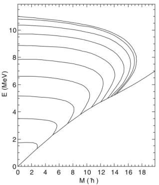
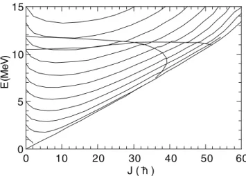
In figure 14 the line of constant level densities are shown in the (E,J) plane for the same nucleus as in figure 13. The yrast
Figure 10. Angular velocity as a function of angular momentum for a rectangular distribution of spin projection (thick lines). The thin lines correspond to a δ-distribution in spin projection. Adapted with permission from [67], Copyright (1974) by Elsevier.
Eγ /Eco
nd
0 0.5 1 1.5 2 2.5 3
J/Jc
0 0.2 0.4 0.6 0.8 1 1.2 1.4
line, which has a weak positive second derivatives, shows a remarkable difference when it is compared with the previ-ously mentioned result for a rectangular spin projection distri-bution. The difference in the dependence of the critical lines as a function of angular momentum is also visible.
2.6. Thermodynamic properties of paired nucleus with fixed number of quasiparticles
The study of relaxation phenomena in nuclei has been widely useful in the description of pre-equilibrium emission of nucle-ons [69–72]. However, one can also forecast many cases where the statistical properties of a fixed quasiparticle system may be of interest. For instance, the coupling of a doorway state (single-particle or collective in nature) with a certain class of particle-hole states needs to be considered in the description of its width. Various relevant thermodynamical quantities will be considered here as a function of the quasiparticle number by using the residual interaction in the form of the pairing approximation, having in mind that for the systems with unre-stricted quasiparticle number, the residual interaction is very important only at low energy [62, 63, 73, 74]. It will be shown that, at small quasiparticle numbers, the pairing correlation is present even at very high excitation energies, which plays a dominant role during the relaxation process leading from a small quasiparticle number to its equilibrium value. The uni-form model, which eliminates the shell effects associated with the fluctuations in the single-particle spacings, is employed to clearly identify the correlation between quasiparticle number and pairing.
2.6.1. Hamiltonian. The same form of pairing Hamiltonian H is used with a constant pairing interaction as in (1). To fix the
mean number of quasiparticle number, a new auxiliary Ham-iltonian is introduced as H=H−ξQ, where Q=2nk is
the quasiparticle number (nk is the quasiparticle occupation number) and ξ is the Lagrange multiplier necessary for this particular constraint. The expectation value of the new Hamil-tonian can be explicitly written as
H=(
k−λ−Ek) +∆
2
G +2
nk(Ek−ξ).
(29)
2.6.2. Grand partition function and other thermodynamic quantities. The grand partition function eΩ=Tre−βH
can be immediately obtained from the Hamiltonian H with
∆
)
J ( h)
∆
J ( h)
J = 4h
δ
T = 0.05885 MeV
δ
= 0.4 MeV
δ∆
J = 4h
δ
T = 0.05903 MeV
δ
= 0.4 MeV
δ∆
Figure 12. Isometric projections of the gap parameter as functions of temperature and angular momentum for the proton and neutron components of 220Rn nucleus. The magnitudes of the scale intervals in the three coordinates are indicated in the figures. Adapted with permission from [68], Copyright (1973) by Elsevier.
T
(M
eV
)
0 0.18 0.36 0.54 0.72 0.90
J ( h )
0 10 20 30 40 50 60
Figure 13. Lines of constant entropy in the (T,J) plane for 220Rn nucleus. The boundaries of the proton and neutron superfluid phases are also shown. The boundary of the superfluid proton component is the one extending farther to the right of the figure. The lowest value of the entropy and the entropy step are both equal to 2.5. Adapted with permission from [68], Copyright (1973) by Elsevier.
)V
e
M(
E
0 5 10 15
J ( h )
0 10 20 30 40 50 60
Ω =−β(k−λ−Ek)−β∆
2
G
+2ln{1+exp[−β(Ek−ξ)]}. (30)
All the other thermodynamical functions for the particle num-ber N, quasiparticle numnum-ber Q, energy E, pairing gap ∆, and entropy S can be obtained by differentiating (30) [67, 75] as
N= 1
β ∂Ω
∂λ = 1− k−λ
Ek tanh
1
2β(Ek−ξ)
,
(31)
Q= 1
β ∂Ω
∂ξ =2
1
1+exp[β(Ek−ξ)],
(32)
E=−∂Ω∂β =k
1−kE−λ k tanh
1
2β(Ek−ξ)
,
(33)
1 Ektanh
1
2β(Ek−ξ) = G
2,
(34)
S=2ln{1+exp[−β(Ek−ξ)]}
+2β Ek−ξ
1+exp[β(Ek−ξ)]. (35) In the graphs presented from here on, the gap parameter will be expressed in terms of the ground-state gap parameter
∆0; the energy and free energy in units of the condensation
energy C=g∆20/2; the temperature in terms of the criti-cal temperature Tc=2∆0/3.5; the quasiparticle number in
terms of the most probable quasiparticle number at the critical temperature Qc=4gTcln2; and the entropy in terms of the
entropy at the critical point Sc=2π2gTc/3.
2.6.3. Limiting properties for T = 0 (β → ∞).
Gap equation. In the limit of β → ∞, the gap equa-tion can be analytically integrated
ξ= 1 2
∆
∆0(∆ + ∆0).
(36)
Quasiparticle number equation. The equation for the quasi-particle number can also be analytically integrated in a similar way, giving
Q=4gξ2−∆2.
(37) Combining the two equations (36) and (37), a relation between Q and ∆ is obtained as
Q=2g
∆
∆0(∆ + ∆0).
(38)
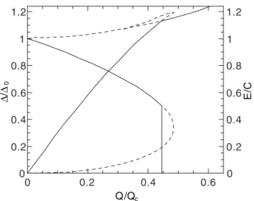
Discussion on the phase stability. Different from the regular dependences of ∆ on both temperature and angular momen-tum, the dependence of ∆ upon Q is anomalous. As shown
in figure 15, ∆ is a triple valued function of Q with one triv-ial and two non-trivtriv-ial solutions in the interval 0QQ∗,
where Q∗= 4 3
1
3g∆0, whereas it is single valued (∆ =0)
for Q > Q*. Starting at ∆ = ∆
0 when Q = 0, the larger
solu-tion decreases as expected down to ∆0/3 at Q = Q*.
Simi-larly, the smaller non-trivial solution starts at ∆ =0 for Q = 0
and increases with Q to coalesce with the larger solution at Q = Q*. This peculiarity must be resolved by deciding which of the three solutions is the stable one.
An immediate test on the two non-trivial solutions can be made by checking the sign of ∂2H/∂∆2. One may recall that
the gap equation, expressed by ∂H/∂∆ =0, represents the
requirement that the Hamiltonian should be stationary with respect to ∆. If ∂2H/∂∆2 is positive, then one has indeed a
minimum, while a negative sign implies that the solution is a maximum. The second derivative calculated at the equilibrium value of ∆ is given as [67]
∂2H ∂∆2 = ∆
21−2nk E3
k −
∆4G 2
1−2nk E3
k
2 .
(39)
By substituting nk with its thermal average and considering the uniform model, one obtains
∂2H
∂∆2 =2g(1−2
∆0−∆ ∆0+ ∆).
(40)
This expression vanishes at ∆ = ∆0/3, which is the value
of ∆ at which the larger and the smaller solutions merge. At
∆>∆0/3 the second derivative is positive, thus indicating a
stable solution, whereas for the values of ∆<∆0/3 the
sec-ond derivative is negative and the solution is unstable.
Energy equation. One must now decide which of the two remaining solutions, the paired or the trivial one (∆ =0), is the stable solution. To do so, let us consider the energy equa-tion, which in the limit of β → ∞ becomes
∆
/
∆0
0 0.2 0.4 0.6 0.8 1 1.2
E/
C
0 0.2 0.4 0.6 0.8 1 1.2
Q/Qc
0 0.2 0.4 0.6
E=−gS2−1
2g∆2+2gξ
ξ2−∆2.
(41)
By subtracting the ground state energy E0=−gS2−g∆20/2
and substituting ξ with its own expression, one obtains the
excitation energy as
E∗= 1
2g(∆20−∆2)(1+∆∆
0) for ∆>0,
(42)
E∗=1
2g∆20+Q 2
8g for ∆ =0.
(43)
The unexpected existence of a first-order phase trans-ition. Shown in figure 15 is the excitation energy as a func-tion of the quasiparticle number. As the gap parameter ∆
decreases from ∆0 to 0, the energy follows a loop. As the
stable solution is the one with the smallest energy, the loop must be bypassed. Since at the bypass point the curves for the paired and the unpaired energies cross. Thus the bypass coordinates can be obtained by equating these two energies
Epaired=Eunpaired or 1
2g(∆20−∆2)(1+∆∆ 0) =
1
2g∆20+Q 2 8g.
(44)
This equation gives ∆x/∆0=1/2,Qx=g∆0/√2, where
∆x and Qx are the values of ∆ and Q at the crossing, respectively. The excitation energy at the crossing is
Ex= (9/8)(g∆02/2) = (9/8)C, where C is the pairing con-densation energy. In conclusion, at Q < Qx the paired solu-tion is the stable one. At Q=Qx,∆ decreases abruptly from ∆0/2 to 0 and remains zero at Q > Qx. This phase transition, clearly first order, is much sharper than the one occurring
at the critical angular momentum, where ∆ continuously
decreases to 0, where the first derivative of ∆ undergoes a
discontinuity.
2.6.4. Properties of the system for T > 0.
Solution of the gap equation. Shown in figure 16 is the dependence of the gap parameter ∆ on the quasiparticle
num-ber Q at various T obtained by simultaneously solving the equations for the gap and quasiparticle number. At T <Tc two
paired solutions exist, whereas at T >Tc there is one paired
solution. Aside from the bending over of the isotherms with
T >Tc (similar to that in figure 15), it appears that the gap
parameter at a fixed quasiparticle number actually increases with T. This is another example of the previously mentioned thermally assisted pairing correlation [26]. An increase in temperature pushes the quasiparticles farther and farther away from the particle Fermi surface, relaxing the blocking due to the quasiparticles and, hence, enhancing the pairing cor-relation. It follows that, for a fixed quasiparticle number, the pairing correlation is not confined to temperatures smaller than the critical one, but actually extends to indefinitely high temperatures.
Free energy and phase stability. In the region of T <Tc, two
paired solutions (plus the usual unpaired solutions) appear. To determine which of the solutions corresponds to a stable sys-tem, the free energy F=−TΩ +ξΩ is investigated, whose dependence upon Q at T<Tc is given in figure 17.
As for T = 0, a loop can be observed, which must be bypassed by the stable solution. This produces a discontinu-ous jump from the paired configuration with a larger ∆ to the
unpaired configuration. This isothermal transition is accom-panied by an energy change ∆E=T∆S, indicating a true first-order phase transition. All of these isotherms present a minimum corresponding to the equilibrium value of Q, which satisfies the condition ∂F/∂Q=ξ=0. This means, when
the number of quasiparticles is not restricted but is allowed to
∆
/
∆0
0 0.25 0.5 0.75 1
Q/Qc
0 0.5 1 1.5 2
Figure 16. Dependence of the gap parameter ∆ upon quasiparticle number Q at various T. The inner isotherm corresponds to T/Tc=
0. The successive isotherms are space at intervals of 0.2T/Tc. The
onset of the first-order phase transition is indicated by an open circle, whereas the unstable solution at the same temperature is indicated by a solid point. Adapted with permission from [75], Copyright (1975) by Elsevier.
attain its equilibrium value, the quasiparticle chemical poten-tial is identically zero.
At T <Tc, the phase transition (first order) occurs for
val-ues of Q larger than the equilibrium value, whereas above Tc,
the phase transition (now second order) occurs for values of Q smaller than the equilibrium value. This information can be used to generate a (T,Q) phase diagram, for example, the one shown in figure 18. This figure shows the boundary between the paired and the unpaired region defined by the vanishing of the gap parameter ∆. At T<Tc this boundary branches
into two lines. The leftmost line corresponds to the continu-ous vanishing of ∆, which does not correspond to any stable
system. The rightmost line corresponds to the discontinuous vanishing of ∆ and is physically significant. The line
char-acterized by ξ=0, corresponding to the equilibrium number of quasiparticles, starts at the origin of the diagram and stays into the paired region up to Tc, when it enters in the unpaired
region. It is along this line that previous pairing calculations have been made [62, 63, 67, 68, 73, 74]. It is useful now to project various quantities on this basic diagram.
Shown in figure 19 are the projected lines of constant gap parameter ∆. It is noticed that, firstly, the gap parameter at
fixed Q actually increases and tends to reach its ground state value as T goes to infinity. Secondly, even for those values of Q for which ∆ =0 at T = 0, an increase in temperature even-tually leads to the onset of pairing, which increases towards the ground state value as an asymptotic limit. These effects are completely understood in terms of the thermally assisted pairing correlation [26, 67, 68].
The (E,Q) diagrams and the plots of various thermodynami-cal quantities. The relevance of constant energy processes in nuclei makes it desirable to use the energy itself as an inde-pendent variable. Shown in figure 20 are the lines of constant
∆ in the (E,Q) plane. The evolution in pairing of a constant energy system can be directly appreciated as it moves from a very low initial quasiparticle number to its equilibrium value. In all the cases of physical interest, the system starts off with a very large pairing gap, close to its ground state value. With increasing the quasiparticle number, the pairing correlation experiences rapidly drops and disappears above the criti-cal energy. The first order phase transition appears as a gap between the two dotted lines.
Level density. Figure 21 shows the (E,Q) plot of the final result of the calculation for the level density, where constant level density lines for a system characterized by g = 7 MeV−1
and ∆0=1 MeV can be seen. The large gap in the plot is
vis-ible due to the first order phase transition.
T/
Tc
0 0.5 1 1.5 2
Q/Qc
0 0.5 1 1.5 2
Figure 18. Phase diagram in the (T,Q) plane. The solid line corresponds to the phase transition (first-order for T<Tc,
second-order for T>Tc) from the paired region (left-hand side) to the
unpaired region (right-hand side). The dotted line corresponds to the paired unstable solution. The line with small and large dots corresponds to the most probable value of Q(ξ=0). Adapted with permission from [75], Copyright (1975) by Elsevier.
T/
Tc
0 0.5 1 1.5 2
Q/Qc
0 0.5 1 1.5 2
Figure 19. Lines of constant gap parameter in the (T,Q) plane. The solid line corresponds to ∆ = 0; the lines to the left correspond to increasing values of ∆ in steps of 0.05 ∆/∆0. Adapted with
permission from [75]), Copyright (1975) by Elsevier.
E/
C
0 1 2 3 4 5
Q/Qc
0 0.5 1 1.5
Figure 20. Lines of constant gap parameter ∆ in the (E,Q) plane. The leftmost line corresponds to ∆/∆0 = 0.05 and the lines to
the right are plotted in intervals of 0.05 ∆/∆0. Adapted with
2.7. Experimental level densities and first-order pairing phase transition
A large body of high-quality low-energy nuclear level-density data are now available in the literature. The stunning, com-mon feature of the level densities, particularly evident for deformed, mid-shell nuclei, is the linear dependence of their logarithm with excitation energy. Above approximately 2∆0,
and up to about the neutron separation energy, they are well described by the constant-temperature expression empirically proposed by Ericson [21], and Gilbert and Cameron [76]
ρ(E)∝exp(E/T),
(45) with the excitation energy E and constant temperature T. This expression turns out to be in good agreement with the cumu-lative number of levels at low excitation energy. However, no fundamental nor quantitative explanation for this relation has been provided. Moreover, the constant-temperature expres-sion is in striking contrast to the expected Fermi-gas behavior predicting a square-root dependence of the level density with excitation energy
ρ(E)∝exp[√2aE],
(46) where a is the level-density parameter.
The experimental linear dependence of the entropy
S(E)≈lnρ(E) given by (45) is the microcanonical hallmark of first-order phase transitions. It implies a constant temper-ature, a latent heat and an infinite heat capacity. As a mat-ter of fact, the experimental data for the rare-earth region [77–83] show that the entropies of adjacent even–even and odd-A nuclei are parallel over the experimental energy range above 2 MeV, that is the level densities of neighboring even– even and odd-A nuclei have nearly identical slopes [84, 85]. This feature allows one to coalesce the level densities of neighboring isotopes by making a horizontal shift along the excitation-energy axis (see figure 22). This shift is constant
with energy and in very good agreement with the even–odd mass difference, which identifies the elementary excitations as the quasi particles. It implies that the energy cost per quasi-particle is constant and independent of excitation energy.
Equally intriguing is the vertical shift between the even–even and odd-A nuclear level densities, merging the lower even–even level density and the higher odd-A one (see figure 22). This dif-ference, approximately constant for excitation energies above approximately 2 MeV, can be interpreted as the entropy car-ried by the extra quasiparticle. Thus, the exper imental evidence alone suggests that, as the system is excited, quasiparticles are created with a constant energy cost and carrying a constant amount of entropy. This theory-independent observation is a clear signature of a first-order phase transition [84, 85]. As will be seen below, the two phases are a superfluid phase and an ideal gas of quasiparticles. Hence, the exper imental data have a thermodynamic interpretation as that of a clear first-order phase transition with latent heat ∆ per (quasi)particle, infinite
heat capacity, and a fixed amount of entropy per (quasi)particle. This interpretation follows from straightforward thermodynam-ics, without recoursing to any specific nuclear structure theory. The phase transition is, at least for nuclei well away from closed shells, clearly related to pairing. First of all, the con-stant shift ∆ is directly related to the liquid drop mass
dif-ference, which, in turn, arises from pairing. Furthermore, by provisionally taking the constant temperature of the exper-imental level-density spectrum to be the BCS critical temper-ature according to the well-known BCS relation (24), one can extract the gap parameter ∆0 and compare it directly with that
obtained from even–odd mass differences represented in the liquid-drop term, namely ∆BM =12A−1/2. From this obser-vation, we can consequently predict the low-energy nuclear level densities from the even–odd mass difference throughout the nuclear chart for regions away from magic proton/neutron
Figure 22. Illustration of constant-temperature level densities. The experimental, horizontal shift gives the slope (1/TCT) through (24), and the vertical shift is related to the entropy excess for the quasiparticle as indicated in the figure. Reprinted from [84]. Non-exclusive license to distribute 1.0.
E (MeV
)
0 5 10 15
Q
0 5 10 15 20
Figure 21. Lines of constant level densities in the (E,Q) plane. The calculation refers specifically to a nucleus with g = 7.0 MeV−1 and with ∆0=1.0 MeV. The lowest level density line has a value
numbers. From these features we can immediately infer that a first-order phase transition with a latent heat takes place at the constant temperature Tc.
We now show that all the empirical features find a close counterpart in the BCS theory. For a set of uniformly spaced single-particle levels, the excitation energy at T =Tc is given
by Ec=g∆20/2+π2gTc2/3, whereas the most probable
num-ber of quasiparticles Qc at Tc is Qc=4gTcln2 [75]. Taking the
ratio of these two quantities and utilizing (24), the average cost per created quasiparticle up to Tc is found as Ec/Qc= ∆0.
This very puzzling result is consistent with the parallel behav-ior of the level densities described above.
Within the BCS theory, we know that at T = 0 the quasi-particle energy is approximately equal to ∆0, and that ∆
decreases with increasing temperature, so that ∆ =0 at
Tc. How is it then possible for the energy per quasiparticle
to be constant in this excitation-energy range? The explana-tion lies mostly in the structure of the quasiparticle energy
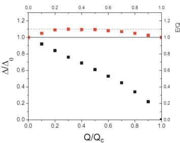
Ek=(k−λ)2+ ∆2. With increasing T, ∆ does indeed decrease, but within the uniform model this is compensated by the increase of the average value of |k−λ| and by the change of the underlying pairing field. For this case, we have calcu-lated the average energy per quasiparticle E/Q as a function of the most probable quasiparticle number for 1<Q<Qc.
Figure 23 shows that the energy per quasiparticle is very close to 1 MeV in the entire region.
The assimilation of T with Tc finds also an explanation
in the BCS model. The dependence of the heat capacity on T exponentially increases from zero and peaks at T =Tc so
that essentially all energy is absorbed at this temperature. This is also true from a microcanonical perspective. From the constant energy cost ∆ per quasiparticle, it follows that the entropy per quasiparticle is
∂S ∂Q =
∆ Tc =
3.53
2 =1.77,
(47)
to be compared with the empirical, vertical shift as discussed above.
The consideration above is based on the BCS theory, which should be revised when applied to finite systems such as nuclei, taking care of large fluctuations owing to the finiteness of the system. In this case the sharp superfluid-normal phase trans-ition is smoothed out and it is not possible to identify a critical temperature Tc. As will be seen later in section 6.2, a
micro-scopic approach including exact pairing is necessary to explain the constant-temperature level density at low excitation energy as well as its Fermi-gas behavior at high excitation energy.
3. Grand-canonical ensemble treatment of pairing problem within the Hartree–Fock–Bogoliubov theory and finite-temperature pairing reentrance
3.1. Hartree–Fock–Bogoliubov theory for hot and hot rotating nuclei
The Hartree–Fock–Bogoliubov theory at finite temperature (HFB) was first derived by Goodman in [33]. This theory, which is generalized from the BCS theory discussed in sec-tion 2, is derived based on the same minimization requirement of the grand potential as the BCS theory, namely δΩ =0, where Ω =E−TS−λN with E, S, λ, and N being the total energy, entropy, chemical potential, and particle number. This variational condition leads to the density operator D given in the form
D= 1
Ze−β(H−λ
ˆ
N),
(48)
whose trace should satisfy the unitarity condition TrD=1
and ∂Ω/∂D=0. In (48), Z=Tr[e−β(H−λˆN)] is the grand
partition function with H being the nuclear many-body Hamiltonian of the form
H=
ij
Tija†iaj+1
4
ijkl
Vijkla†ia†jalak,
(49)
where Tij is the kinetic energy operator and vijkl is the anti-symmetrized matrix elements of the two-body interaction. Within the HFB, the Hamiltonian (49) is often expressed in terms of the independent-quasiparticle Hamiltonian HHFB,
namely
H−λNˆ ≈HHFB=E0+
i
Eiαi†αi,
(50)
where E0 is the ground-state energy, Ei is energy of the quasi-particle, and α†i(αk) is the quasiparticle creation (destruction) operator obtained from the Bogoliubov transformation. The latter is expressed in terms of a matrix form
α†
α
=
U V
V∗ U∗ a†
a
,
(51)
where the coefficients U and V of the Bogoliubov transfor-mation must satisfy the conditions UU†+VV†=1 and Figure 23. Average energy per quasiparticle as a function of the
![Figure 17. Example of an isothermal free energy loop. Adapted with permission from [75], Copyright (1975) by Elsevier.](https://thumb-us.123doks.com/thumbv2/123dok_us/8200762.2174282/13.892.77.442.90.387/figure-example-isothermal-energy-adapted-permission-copyright-elsevier.webp)