STATISTICAL CONTRIBUTIONS TO NON-EXPERIMENTAL STUDIES
Byeongyeob Choi
A dissertation submitted to the faculty at the University of North Carolina at Chapel Hill in partial fulfillment of the requirements for the degree of Doctor of Philosophy in the Department
of Biostatistics in the Gillings School of Global Public Health.
Chapel Hill 2015
Approved by:
ABSTRACT
Byeongyeob Choi: Statistical contributions to non-experimental studies (Under the direction of Jason P. Fine and M. Alan Brookhart)
ACKNOWLEDGMENTS
TABLE OF CONTENTS
LIST OF TABLES . . . ix
LIST OF FIGURES . . . xi
CHAPTER 1: INTRODUCTION AND LITERATURE REVIEW . . . 1
1.1 Introduction . . . 1
1.2 Instrumental variable methods . . . 5
1.2.1 Complete data . . . 5
1.2.2 Right-censored outcome data . . . 8
1.3 Negative control outcomes . . . 13
1.3.1 Detection of unmeasured confounding . . . 13
1.3.2 Control outcome calibration . . . 15
CHAPTER 2: TWO-STAGE ESTIMATION OF STRUCTURAL INSTRUMENTAL VARIABLE MODELS WITH COARSENED DATA . . . 17
2.1 Introduction . . . 17
2.2 General Framework for Coarsened Data . . . 20
2.2.1 Model and estimation . . . 20
2.2.2 A resampling method for variance estimation . . . 25
2.3 Inference . . . 26
2.3.1 Case 1-1: Fully-observed continuous exposure . . . 28
2.3.2 Case 1-2: Right or left-censored exposure . . . 30
2.3.3 Case 2-1: Dichotomized exposure via coarsening of latent exposure . . . 33
2.4 Simulation study . . . 41
2.5 SEER Colon Cancer Data . . . 43
2.6 Discussion . . . 49
2.7 Proofs . . . 51
CHAPTER 3: A NEW INSTRUMENTAL VARIABLE ESTIMATOR USING A NEGATIVE CONTROL OUTCOME . . . 66
3.1 Introduction . . . 66
3.2 A new instrumental variable estimator with a negative control outcome . . . 67
3.3 A Test for Instrumental Variable Assumption and Combined Instrumental Variable Estimator . . . 76
3.4 Simulations . . . 84
CHAPTER 4: SENSITIVITY ANALYSIS FOR AN EXPOSURE EFFECT WITH A NEGATIVE CONTROL OUTCOME WHEN UNOBSERVED CONFOUNDERS MAY BE PRESENT . . . 91
4.1 Introduction . . . 91
4.2 Methods . . . 93
4.2.1 Control outcome calibration approach . . . 93
4.2.2 Marginal model approach . . . 97
4.2.3 Conditional likelihood approach . . . 106
4.3 Simulations . . . 110
CHAPTER 5: PRACTICABLE CONFIDENCE INTERVALS FOR CURRENT STATUS DATA . . . 118
5.1 Introduction . . . 118
5.2 Nonparametric confidence interval methods . . . 119
5.3 Simulations . . . 123
5.4 Real examples . . . 126
5.4.1 Mice lung tumor data . . . 126
5.5 Conclusion . . . 132
LIST OF TABLES
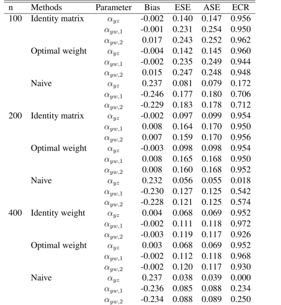
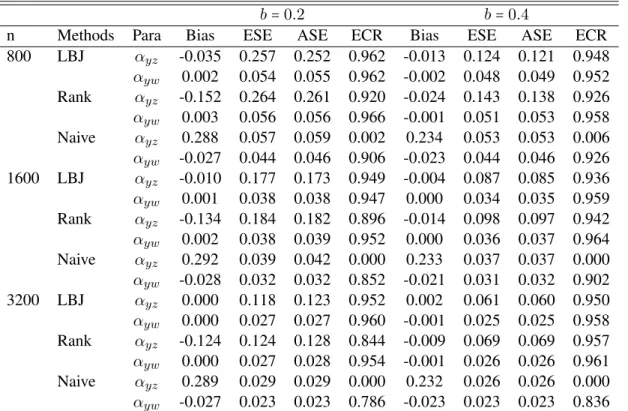
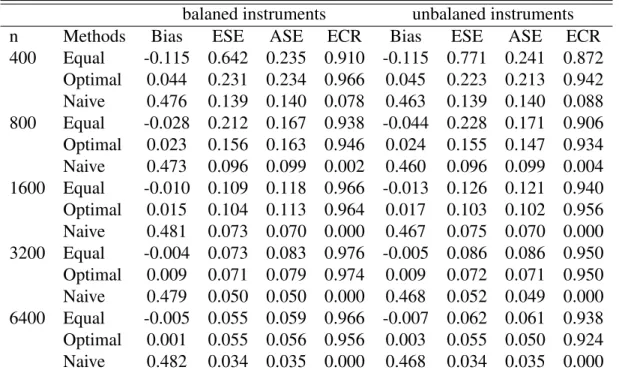
2.1 Results for Case 1-1 (NN): empirical bias (Bias), empirical standard error (ESE), average of the estimated standard error (ASE) and empirical coverage rate (ECR) of 95%
Wald-type confidence interval. . . 44 2.2 Results for Case 1-2: empirical bias (Bias), empirical
standard error (ESE), average of the estimated standard error (ASE) and empirical coverage rate (ECR) of 95%
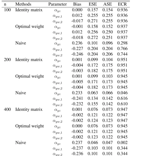
Wald-type confidence interval. . . 45 2.3 Results for Case 2-1: empirical bias (Bias), empirical
standard error (ESE), average of the estimated standard error (ASE) and empirical coverage rate (ECR) of 95%
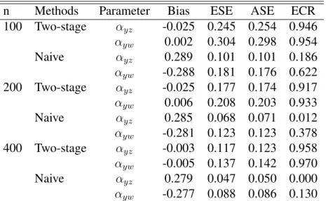
Wald-type confidence interval. . . 46 2.4 Results for Case 2-2: empirical bias (Bias), empirical
standard error (ESE), average of the estimated standard error (ASE) and empirical coverage rate (ECR) of 95%
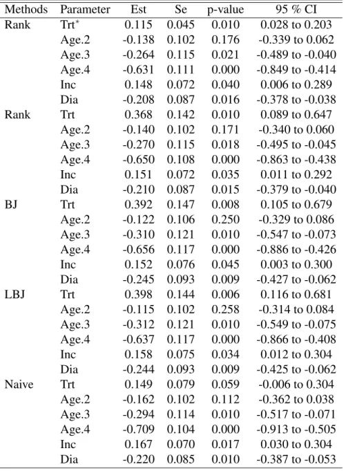
Wald-type confidence interval. . . 47 2.5 Estimates (Est), Standard errors (Se), p-values (p-value)
and 95% Wald confidence intervals (95% CI) for the
parameters in the SEER data. . . 50
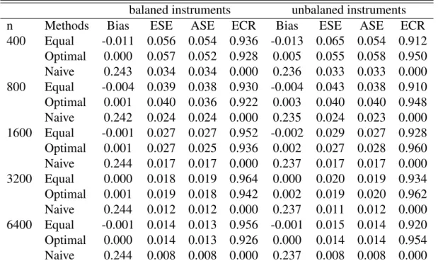
3.1 Results for continuous exposure: empirical bias (Bias), empirical standard error (ESE), average of the estimated standard error (ASE) and empirical coverage rate (ECR)
of 95% Wald-type confidence interval. . . 87 3.2 Results for binary exposure: empirical bias (Bias), empirical
standard error (ESE), average of the estimated standard error (ASE) and empirical coverage rate (ECR) of 95%
Wald-type confidence interval. . . 88 3.3 Results for the combined estimator: strength of unmeasured
confounding (Strength), empirical bias (Bias), empirical standard error (ESE), average of the estimated standard error (ASE) and empirical coverage rate (ECR) of 95%
3.4 Results for the test: power of the test (Power), empirical bias (Bias), empirical standard error (ESE), average of the estimated standard error (ASE) and empirical coverage
rate (ECR) of 95% Wald-type confidence interval. . . 90
4.1 Sensitivity parameter values used in simulations. . . 112
4.2 Logistic regression model with(a, b) = (0.5,0.4) . . . 113
4.3 Logistic regression model with(a, b) = (1.0,0.8) . . . 114
4.4 Proportional hazard model with(a, b) = (0.5,0.4) . . . 115
4.5 Proportional hazard model with(a, b) = (1.0,0.8) . . . 116
LIST OF FIGURES
1.1 Causal diagram showing an ideal negative control outcome N for use in identifying potential unmeasured confounding. N should have the same incoming arrow as outcome Y,
except that N is not caused by Z. . . 14
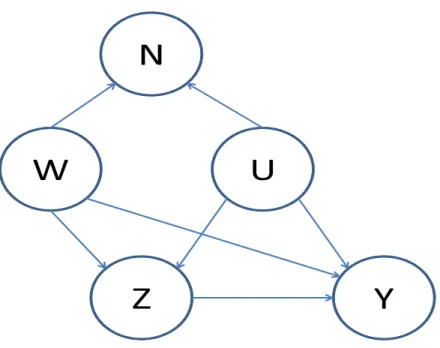
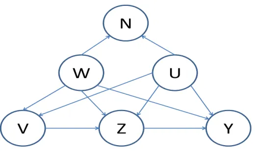
3.1 Causal diagram showing an ideal negative control outcome N for use in estimating an exposure effect on an outcome with an instrument V. N should have the same incoming arrow as an outcome Y, except that N is not caused by Z. V can be caused by measured and unmeasured
confounders W and U. . . 68
5.1 (a): Three observation time distributions (exp(1),gamma(3,1/3) and unif(0,2)) used in simulations. (b) and (c): Mice
data, kernel density estimates for observed death time in conventional environment and germ-free environment. (d): Menopause data, kernel density estimates for observed
age in years . . . 126 5.2 Mice lung tumor data. Four types of confidence intervals
for conventional environment (the first row) and germfree environment (the second row). From the left, the Wald CIs, the logit-transformed Wald CIs, the log(-log) transformed Wald CIs, the nonparametric bootstrap CIs and the bootstrap-Wald CIs. The estimates of NPMLE for the distribution function
of time to lung tumor onset are plotted at observed death times and the corresponding confidence intervals
are plotted with vertical lines. . . 128 5.3 Menopause data. Four types of confidence intervals for
operative menopause (the first row) and natural menopause (the second row). From the left, the Wald CIs, the logit-transformed Wald CIs, the log(-log) transformed
Wald CIs, the nonparametric bootstrap CIs and the bootstrap-Wald CIs. The estimates of NPMLE for the cumulative incidence rate of menopause are plotted at observed ages and the corresponding confidence intervals are plotted with
CHAPTER 1: INTRODUCTION AND LITERATURE REVIEW
1.1 Introduction
Researchers in epidemiology often have an interest in making a causal inference for an exposure effect on an outcome. In many cases, observation studies are employed to do such an inference. However, observation studies are easily affected by unmeasured confounders, which may result in a biased estimate of the exposure effect due to residual confounding. In economic terminology, we say the exposure variable is endogenous in this case and classical statistical methods adjusting measured confounders fail to give correct inference results for the the exposure effect.
An instrumental variable (IV) analysis is designed to overcome the unmeasured confounding problem (Brookhart et al. 2006, McClellan et al. 1994, Schneeweiss et al. 2006, Stukel et al. 2007). Although the requirements of an IV depend on a particular analytic method one chooses, we can say that a variable is an IV if it satisfies the following three conditions (Brookhart et al. 2010): (i) it has a causal effect on the exposure; (ii) it has effects on the outcome only through the exposure; (iii) it is unrelated to an unmeasured confounder. A typical example of an IV is a randomized indicator, which is usually available, to estimate a drug effect in randomized trial with non-compliance.
(1974) proposed nonlinear two-stage least squares (NL2SLS), which generalizes 2SLS for nonlinear models. Newey (1990) pointed out the asymptotic efficiency of IV estimators of nonlinear model depends on the form of instruments. He proposed efficient instrumental variables estimation of nonlinear models, which employs nonparametric estimation of the optimal instruments. Abadie (2003) introduced a new class of IV estimators for linear and nonlinear treatment response models. Terza et al. (2008) introduced two-stage predictor substitution (2SPS) estimation and two-stage residual inclusion estimation (2SRI) for nonlinear models. 2SPS is the extension to nonlinear models of 2SLS. 2SRI is similar to 2SPS except that first stage residuals are included as additional regressors instead of replacing the endogenous variables by their predicted values. They showed that in a generic parametric framework, 2SRI is consistent and 2SPS is not. In case where either response or exposure is incompletely observed, however, such semiparametric methods are not applicable. An important special case of coarsened data occurs with time to event outcomes and exposures, which may be subject to both censoring and truncation.
In the case where we do not have a tool such a valid IV, thus it is hard do find a reliable way to consistently estimate the parameters, it is desirable to evaluate the sensitivity of regression results to unmeasured confounders. There have been several developed sensitivity analysis techniques (Rosenbaum and Rubin 1983, Lin et al. 1998, Brumback et al. 2004, Gustafson et al. 2010, VanderWeele et al. 2012). Among those, the methods of Lin et al. (1998) are applicable to general regression models and can be easily performed (VanderWeele 2008). Lin et al. (1998) assumed that the distribution of the unmeasured confounder conditional on the measured confounders and the exposure is normal or binomial, and they identified simple algebraic relationships between a true exposure effect in the full model and an apparent exposure effect in the reduced model which does not control for unmeasured confounders. One can make an inference on the true exposure effect by making a simple adjustment to the estimate and the confidence interval of the apparent exposure effect. Lin et al. (1998) developed their method for linear, log-linear, logistic and proportional hazard models.
(Flanders et al. 2011, Lipsitch et al. 2010, Lumley and Sheppard 2000, Jackson et al. 2006, Smith 2008; 2012). An outcome is said to be a valid negative control outcome(N)if it is influenced by measured confounders(W)and an unmeasured confounder(U)in the association between the exposure(Z)and the main outcome(Y), but not directly influenced by the exposure (Lipsitch et al. 2010). Those conditions are sufficient to detect unmeasured confounding, but insufficient to estimate the causal effect. Tchetgen Tchetgen (2014) made a more progress to estimate the causal effect by imposing an additional assumption that the negative control outcome is independent of a treatment received conditional on the measured confounders and counterfactual outcomes. This assumption implies that the counterfactual outcomes are ideal proxies of the unmeasured confounders. Under this assumption, an additive causal effect on a continuous outcome can be estimated by regressingN onto(W, Y, Z).
Herein, we develop IV methods to estimate the causal effect of the exposure in coarsened data. The developed methods are focused on right-censored outcome data. Further, we develop a new IV estimator with a negative control outcome, which is consistent even if the IV assumption that the IV should be independent of an unmeasured confounder is violated. For the case where the IV is not available, we develop the method for sensitivity analysis with a negative control outcome under unmeasured confounding. Finally, we introduce improved confidence intervals for current status data. The remainder of this chapter provides the review of the IV methods for linear and nonlinear models with complete and incomplete data and that of the methods with a negative control outcome.
that we consider.
1.2 Instrumental variable methods
1.2.1 Complete data
First, we discuss linear models. Fori=1, ..., n, letyi be the response, letzi be the exposure
which is endogenous, letvi be thep×1vector of the instrumental variables (IVs) and letwi be
theq×1vector of the confounders. The linear model for the response is given by
yi =αo+αyzzi+αααTywwi+εi. (1.1)
In this model,αyz represents the average causal effect ofz ony. The usual estimation methods
do not give consistent estimators for the regression parameters in (1.1) because z and ε are correlated. The linear model for the exposure is given by
zi=βo+βββTzvvi+βββTzwwi+ηi.
In matrix notation, we can write
y=Xααα0+εεε,
z=Dβββ0+ηηη,
whereααα0 = (αo, αyz, αααyw)T,βββ0 = (βo, βββzv, βββzw)T, andy, z, εεεandηηηare n-vectors with typical
elementyi,zi,εiandηi, andXandDaren×(2+q),n×(1+p+q)matrices with row(1, zi,wi)
and(1,vi,wi).
We assume thatE(ε∣v) = E(η∣v) = 0, var(ε∣v) = σ2
ε, var(η∣v) = ση2 andE(εη∣v) = σεη.
We also assume that the probability limit of DTD/n and XTX/n are given by Σ
D and ΣX
The two-stage least squares (2SLS) estimator forααα0 is
ˆ α α
α2sls= (XTD(DTD)−1DTX)−1(XTD(DTD)−1DTy).
The 2SLS can be also obtained by applying least squares to (1.1), where zi is replaced by its
predicted value. The 2SLS is the value ofαααto minimize
(y−Xααα)TD(DTD)−1DT(y−Xααα),
The 2SLS is consistent and the limiting distribution of√n(αααˆ2sls−ααα0)is normal with mean
zero and variance(βββTΣ
Dβββ)−1σ2ε. If we have one IV and no confounders, then the 2SLS for the
parameter of the exposure effect,αyz, is the ratio of the sample covariances,cov̂(y, v)/ ̂cov(z, v).
Next, we discuss non-linear models. Let consider the following nonlinear regression model,
yi =f(zi,wi, ααα) +εi,
where f is a possibly nonlinear function in z, w and ααα. Endogeneity occurs because of the correlation of z and ε. For Amemiya’s nonlinear two-stage least squares (NL2SLS) Amemiya (1974), f is assumed to have continuous first and second derivatives with respect to ααα. The NL2SLS estimator (Amemiya 1974) ofαααis the value ofαααthat minimizes
Φ(ααα) = (y−f)TH(HTH)−1HT(y−f),
whereyandf aren-component vectors whoseith elements areyi andf(zi,wi, ααα)respectively,
andHis an×K matrix of certain constants with rankK ≤ (1+p+q). IfH=D, then NL2SLS reduces to 2SLS. The NL2SLS is consistent for the true valueααα0 and under certain conditions
√
n(αααˆnl2sls−ααα0)is normal with mean zero and variance
σε2{plimn→∞1 n ˙
f(ααα0)TH(HTH)−1HTf˙(ααα0)}
−1
wheref˙(ααα)is the first derivative off(ααα)with respect toααα.
Terza et al. (2008) assume the regression model of the responseyis of the form
yi=M(αyzzi+αααTywwi+αyuui) +ei, (1.2)
whereM(⋅) is a known nonlinear function, uis an unmeasured confounder and eis a random error tautologically defined as e = y−M(αyzzi +αααywwi +αyuui) so that E(e∣z,w, u) = 0.
Endogeneity occurs because of the correlation between z and u. They assume the regression model of thezis of the form
zi =r(βββTzvvi+βββTzwwi) +ui, (1.3)
whereris a known nonlinear function.
The 2SPS method is straightforward to implement. In the first stage, we obtain consistent estimates of(βββzv, βββzw),(βββˆˆˆzvzvzv,βββˆˆˆzwzwzw), by applying the nonlinear least squares (NLS) method to the
model (1.3). Then, compute the predicted values of zi, zˆi = r(βββˆ T
zvvi+βββˆ T
zwwi), fori = 1, ..., n.
Correspondingly, define the residuals uˆi =zi−zˆi. In the second stage, estimate the parameters
(γyz, γγγyw)by applying NLS to the model
yi=M(γyzzˆi+γγγTywwi) +e2SPSi , (1.4)
where e2SPS
i is the regression error term. The resultant estimate, (γˆyz,γγˆˆˆγyw), is the estimate of
(αyz, αααyw).
The 2SRI estimation is performed by including the residual, u, in the second stage model.ˆ We apply NLS to the following model,
yi =M(αyzzi+αααywT wi+αyuuˆi) +e2SRIi , (1.5)
in the context of two-stage optimization estimator (Newey and McFadden 1994, White 1994, Wooldridge 2002). For linear models, 2SPS and 2SRI are equivalent to 2SLS.
1.2.2 Right-censored outcome data
Several IV methods for right-censored outcome data have been proposed. Robins and Tsiatis (1991) developed IV estimators to correct for non-compliance in randomized trials by estimating the parameters of a class of semiparametric failure time models, the rank preserving structural failure time models (RPSFTM), using a class of rank estimators. In a randomized clinical trial designed to study the effect of a drug on survival, subjects are assigned to treatment protocols. Unfortunately, some subjects often fail to comply with their assigned regimes. The method of Robins and Tsiatis (1991) allows one to estimate the true treatment effect, i.e., the effect that would be observed if all subjects complied with their assigned protocols, in the presence of such non-compliance.
Fori=1, ..., n, supposezi is a treatment indicator,hi(t) = {zi(u); 0 ≤u≤t}is a treatment
history, vi is a randomization group indicator and ui is the survival time if the ith subject was
never to receive treatment, i.e., zi(t) = 0 for all t. Robins and Tsiatis (1991) assumed U is
independent of the treatment arm to which the subject is assigned. In the absence of censoring, we observe the random variables(Ti, Hi(Ti), Vi), whereTiis the observed failure time of theith
subject.
A RPSFTM relatesUi to{Ti, H(Ti)}by assuming
Ui =ψ(Ti, Hi(Ti), ααα0),
where ααα0 ∈ Rp is an unknown parameter and ψ(⋅) is a known smooth function. A simple
form ofψ(Ti, Hi(Ti), ααα0)is
´Ti
0 exp(α0Zi(x))dx. Theψ(⋅)is assumed to satisfy the following
conditions.
1, ..., p)and almost alltwith respect to Lesbesque measure whereψt(t, h(t), ααα) =∂ψ(t, h(t), ααα)/∂t,
ψαj(t, h(t), ααα) =∂ψ(t, h(t), ααα)/∂αj andψt,αj(t, h(t), ααα) =∂ψt(t, h(t), ααα)/∂αj.
Monotonicity:ψ(t, h(t), α) >ψ(u, h(u), α)ift>u. Identity:ψ(t, h(t),0) =t
Independence and Indentification: There exists a uniqueα0such that
U(α0) ⊥⊥V,
whereU(α) =ψ(T, H(T), α)andA⊥⊥B meansAandB are independent.
DefineNi(u, ααα) =I(Ui(ααα) ≤u)andYi(u, ααα) =I(Ui(ααα) ≥u), whereI(A) =1if statementA
is true andI(A) =0otherwise. Given a knownp-vectorg(v, u, ααα) = {g1(v, u, ααα), ..., gp(v, u, ααα)}T,
Sn(ααα,g)is defined to be thep-vector with components
Sn,j(ααα,g) = n
∑
i=1
ˆ
dNi(u, ααα){gj(Vi, u, ααα) −g¯j(u, ααα)}, j=1, ...., p,
where
¯
gj(u, ααα) = n
∑
i=1
gj(Vi, u, ααα)Yi(u, ααα)/ n
∑
i=1
Yi(u, ααα).
Letαααˆ(g)be a value ofαααthat solvesSn(α,αα g) =0. SinceSn(ααα,g)is a step function inααα, we
obtainαααˆ(g)by minimizingαααˆ(g)Tαααˆ(g). The consistency and asymptotic normality ofαααˆ(g)can
be proven by the asymptotic theory of rank estimators of a linear regression (Tsiatis 1990). Robins and Tsiatis (1991) considered the restrictive type of censoring. They assumed the censoring time C is known for all subjects. The observable variables (Ti, H(Ti), Vi, Ci) are
assumed to be i.i.d. and (U(ααα0), C) ⊥⊥ V. For a valid inference onααα, a new censoring time
needs to be defined and this complicates the inference.
a distribution for these transformed failure times. Instrumental variable linear rank estimator (IVLR) is proposed, which exploits the fact that for the true GAFT, the IV does not influence the hazard of the transformed failure times. However, like the method of Robins and Tsiatis (1991), censoring times should be known for all subjects and a new censoring time needs to be defined.
Brannas (2000) assumed accelerated failure time (AFT) models. The estimators proposed are IV adaptations to the Powell symmetrically trimmed least squares and the Buckley-James estimators for right-censored data. That is, he applied those two estimation methods to the AFT models where the endogenous variable is replaced by its predicted values. Simulation studies showed that they perform well, however, the theoretical properties of these procedures were not investigated.
Loeys and Goetghebeur (2003) proposed a causal proportional hazards estimator for the effect of treatment actually received in a randomized trial with all-or-nothing compliance. Suppose that n independent subjects were randomized over experimental treatment (Vi = 1) or control
(Vi =0). For subjection treatment (respectively control), all-or-nothing exposure to treatment
Z1i (Z0i) is observed, along with its possibly right-censored survival timeT1i (T0i). They make
the following assumptions.
(A1) (Z1i, T1i, Z0i, T0i, Vi) are i.i.d. random variables, implying potential outcomes for each
person are unrelated to the treatment or outcome of other individuals. (A2) The randomization assumption: (Z1i, T1i, Z0i, T0i) ⊥⊥Vi.
(A3) No access to experimental therapy on the control arm. Hence, Z0i equals to 0 for all
subjects, andT0irepresents the treatment-free outcome, when randomized to control.
(A4) Following (A3), we also require that P(T1i > t∣Z1i = 0) = P(T0i > t∣Z1i = 0). This
assumption is called the “absence of indirect effect" by Pearl (2002) and “the exclusion restriction" by Angrist et al. (1996).
They use the following causal proportional hazard model,
In (1.6),exp(α0)captures the causal proportional hazards effect within the treatable subpopulation.
The interest here is to estimateexp(α0).
Let Ci be a censoring time for the ith subject, T˜i = min(Ti, Ci), δi = I(Ti ≤ Ci), Ni(t) =
I(T˜i≤t, δi=1),Yi(t) =I(T˜i ≥t)and filtration
mathbbFt = σ{Ni(s), Yi(s+), Vi, Zi, i = 1, ..., n; 0 ≥ s ≥ t}. They model intensity process as
follows.
E{dNi(t)∣Vi(1−Zi) =1, Yi(t)} =λ00(t)Yi(t)dt
E{dNi(t)∣Vi=0, Yi(t)} = {(1−π(t))λ00(t) +π(t)λ01(t)}Yi(t)dt
E{dNi(t)∣ViZi=1, Yi(t)} =λ01(t)eαYi(t)dt,
whereπ(t) =P(Z1i=1∣T˜i≥t, Vi =0). For knownπ(t), we could then define
dΛˆ01(t) =
1 π(t) {∑i
(1−Vi)dNi(t)
∑jYj(t)(1−Vj) − (
1−π(t)) ∑
i
Vi(1−Zi)dNi(t)
Yj(t)Vj(1−Zj) }
(1.7)
If we substitute (1.7) into (1.6), then we obtain the following score equation,
∑
i
ˆ
dNi(t) [ViZi− {∑ j
ViZieαYj(t)}
1 π(t) × {
1−Vi
∑jYj(t)(1−Vi) −
(1−π(t))Vi(1−Zi)
∑jYj(t)(1−Zi)Vi }] =
0
(1.8)
For givenπ(t), the process (1.8) has compensator 0, and the martingale central limit theorem can be used to obtain asymptotic normality of the resultant estimator. However,π(t)is unknown by (A3). Therefore, (1.8) should be estimated. The authors estimate S01(t) with monotonic
decreasing assumption and its jump is used fordΛˆ01(t).
Loeys et al. (2005) extended the methods of Loeys and Goetghebeur (2003) to allow more general exposure level and covariates in the model. The model they considered is
whereUiis a subjecti’s potential exposure to the experimental treatment if he/she were randomized
to treatment andXi is a covariate vector for theith subject. The challenging here is that Ui is
unobserved for all subjects in the control group ({Vi = 0}). The estimation procedures relies
heavily on randomization.
We rewrite the model (1.9) in terms of survival distribution,
S(t∣Vi=1, Ui=u,Xi=x) =S(t∣Vi =0, Ui=u,Xi=x)exp(α0u). (1.10)
Now, survival probability in the control group are a mixture of unobserved compliance-specific probabilities, i.e.S(t∣Vi=0,Xi=x)equals
∑
u
S(t∣Vi=0, Ui =u,Xi =x)P(Ui=u∣Vi =0,Xi=x), (1.11)
whenUi is discrete. If the model (1.10) holds, the model (1.11) also equals
∑
u
S(t∣Vi =1, Ui=u,Xi=x)exp(−α0u)P(Ui=u∣Vi =1,Xi =x),
sinceP(Ui=u∣Vi =0,Xi=x) =P(Ui=u∣Vi=1,Xi=x)by definition ofUiand randomization.
We defineSˆ1→0(t∣x;α)as
ˆ
S(t∣Vi=1, Ui =u,Xi =x)exp(−α0u)Pˆ(Ui =u∣Vi=1,Xi=x).
The unknown parameterαis estimated by the value ofαthat minimizes the distance between the ˆ
S1→0(t∣x;α) and the fitted treatment-free survival distribution in the control group conditional
on X. To this end, they propose a logrank test which is built as a sum of x-specific pseudo martingales in the control group:
∑
Vi=0
whereΛˆ1→0(T˜i∣xi;α) = −log ˆS1→0(T˜i∣xi;α). The variance of (1.12) can be estimated by2∑Vi=0
ˆ
Λ1→0(T˜i∣xi;α).
The point estimator forα0 can be found as theα-value that minimizes theχ2 value of the test
statistic
( ∑
Vi=0
{δi−Λˆ1→0(T˜i∣xi;α)}) 2
/ (2 ∑
Vi=0
ˆ
Λ1→0(T˜i∣xi;α)).
The proposed methods in Chapter 2 is based on AFT model like Robins and Tsiatis (1991), Bijwaard (2008) and Brannas (2000). Unlike Brannas (2000), our methods are theoretically well justified with consistency and asymptotic normality. Furthermore, our methods do not need the condition that the consorting times are known for all subjects as in Robins and Tsiatis (1991) and Bijwaard (2008).
1.3 Negative control outcomes
1.3.1 Detection of unmeasured confounding
Lipsitch et al. (2010) provides a comprehensive review of the use of negative controls to identify confounding in observations studies. They establish the conditions under which negative control outcomes and negative control exposures can be used to detect unmeasured confounders. Here we focus on the negative control outcomes.
A negative control outcome (N) should be an outcome that are affected by the set of measured (W) and unmeasured (U) confounders of the association between the exposure (Z) and the outcome (Y). We say such N is an “U-comparable" outcome. If N is not caused by Z, then any association of N and Z observed by the same analysis method which is used to determine the association of Y and Z would indicate the bias in that of Y and Z.
z
h
t
E
may satisfy “U-comparable" because protective effect of vaccination should be specific to influenza season and it may share the common confounders with mortality or pneumonia/influenza hospitalization during influenza season.
Jackson et al. (2006) also used irrelevant outcomes to influenza vaccination such as hospitalization for injury or trauma as negative control outcomes. They postulated that the effect of influenza vaccination is specific to the outcome related to influenza. They found that there was also protective effects on injury or trauma hospitalization. This indicates that the observed effectiveness of vaccination is biased due to uncontrolled confounders.
1.3.2 Control outcome calibration
Tchetgen Tchetgen (2014) developed control outcome calibration approach to estimate an exposure effect on an outcome under unmeasured confounding. His key assumption is that a negative control outcome is independent of treatment selection conditional on measured confounders and counterfactual outcomes. This assumption implies that counterfactual outcomes are ideal proxy measures for an unmeasured confounder.
Let Yz denote a main outcome for the subject who received the treatmentz. Also, let Nz
denote a negative control outcome for the subject who received the treatmentz. Definition 1 of Tchetgen Tchetgen (2014) says thatN is a negative control outcome ifNz =N (z =0,1)for all
individuals and the confounding variables for the exposure-negative control outcome association are the same as those for the exposure-main outcome association.
LetYZ = {Yz ∶ z ∈ Z} denote the set of all counterfactuals for the main outcome under all
possible values of the exposure in the setZ. Then, Assumption 1 of Tchetgen Tchetgen (2014)
says that the exposure is independent ofNz conditional on{W,YZ}, or
N =Nz⊥⊥Z∣ {W,YZ}.
Tchetgen Tchetgen (2014),
N ⊥⊥Z∣ {W, Y(Ψ)},
if and only ifΨ=Ψ0. Using a linear regression model, we can set
E(N ∣Z, W, Y(Ψ0) =E(N ∣W, Y(Ψ0))
=β1+β2TW +β3Y(Ψ0),
=β1+β2TW +β3Y +β4Z,
whereβ4 = −β3Ψ0, assuming that β3 ≠ 0. Thus the estimator of Tchetgen Tchetgen (2014) is
give by
ˆ
CHAPTER 2: TWO-STAGE ESTIMATION OF STRUCTURAL INSTRUMENTAL VARIABLE MODELS WITH COARSENED DATA
2.1 Introduction
Observational studies are subject to confounding by variables which affect an exposure and an outcome. Confounding is one of major reason to yield biased estimates in observational studies. Regression adjustment or propensity score methods are usually used to overcome this problem. However, those methods require that all of the confounders are observed and this may not be the case in many cases. In economic terminology, we say the exposure variable is endogenous when the exposure is correlated with an error term by sharing unmeasured confounders. Endogeneity often occurs in randomized trials as well when there is non-compliance, which becomes problematic if it is caused by unobserved variables that are risk factors for the outcome. In that case, the usual regression estimators may not be consistent.
Instrumental variable method is an approach to yield unbiased estimate of the endogenous exposure. Although, the requirements of an IV depend on a particular analytic method one uses, the following three conditions are sufficient to define the IV (Brookhart et al. 2010): (i) an IVV has a causal effect on the exposure Z, (ii)V affects the outcome Y only throughZ, (iii) V is unrelated to an unmeasured confounder U. In randomized trials, a randomization assignment indicator is often used as an IV to construct IV estimators for meaningful casual effects of treatment on the outcome (Robins and Tsiatis 1991, Loeys and Goetghebeur 2003, Loeys et al. 2005, Nie et al. 2011).
equation (exposure model) relates Z to V and W linearly. The regression parameters in the outcome model are identified using the instrument. For the case of no confounders, an IV estimator is given as the ratio of two covariance estimators,cov̂(Y, V)/ ̂cov(Z, V). For the case where there are confounders, generalized method of moments (Hansen 1982) or two-stage least squares (Theil 1953) are used.
There has been considerable work with complete data, where both outcome and exposure are fully observed and assumed to satisfy semiparametric linear or nonlinear or nonparametric structural equation models with unspecified error distributions (Theil 1953, Amemiya 1974; 1982, Newey 1990, Chen and Portnoy 1996, Newey et al. 1999, Newey and Powell 2003). The popular two-stage least squares estimator has an explicit form, with a well-characterized sampling distribution and plug-in variance estimation, making inference straightforward (Bollen 1996, Bollen et al. 2007). However, if either response or exposure are incompletely observed, such semiparametric methods are not applicable. There has been limited work addressing two-stage IV estimation with such coarsening.
If we observe only a subset of the complete-data sample space where true data lie, then we refer to this kind of data as coarsened data (Heitjan and Rubin 1991). The various ways of coarseness include missing, rounding, heaping, right-censoring and so on. In this article, we focus on right-censored data, however, other types of coarsened data such as truncated data can be analyzed with our methods. Our methods do not cover coarsened data such as age heaping, whose valid inference is achieved by multiple imputation (Heitjan and Rubin 1990).
censoring due to dropout and other coarsening are not permitted. Bijwaard (2008) extended Robins and Tsiatis (1991) to generalized accelerated failure time models under similar censoring assumptions. Loeys and Goetghebeur (2003) proposed the IV estimators for the effect of treatment actually received in a randomized trial with all-or-nothing compliance based on the proportional hazard models. These methods were extended to allow more general exposure level and covariates to be included in the causal proportional hazard model (Loeys et al. 2005). Nie et al. (2011) proposed the IV estimators for the effect of treatment on survival probability in randomized trials with noncompliance and administrative censoring, which are extensions of the methods of Baker (1998). Br¨ann¨as (2000) considered ad hoc two-stage estimators for the standard linear structural equation models which are IV adaptations of the symmetric trimmed least squares (Powell 1986a) and the Buckley-James (Buckley and James 1979) estimators for right censored data. However, the theoretical properties of these procedures were not investigated and a rigorous investigation of two stage IV estimation in linear models with right censoring is not apparent in the literature.
In Section 3, we discuss details related to the implementation of our semiparametric estimator when either response or exposure may be censored, employing existing estimators for accelerated failure time models under censoring. These methods are shown to perform well in simulations reported in Section 4, where naive estimation which ignores the unmeasured confounded may produce severely biased estimates of exposure effects. The practical utility of the methods is illustrated in a study of the comparative effectiveness of colon cancer treatments, where the effect of treatment on survival is confounded by patient health status.
2.2 General Framework for Coarsened Data
2.2.1 Model and estimation
For i = 1, ..., n, suppose that Yi is the response variable, Zi is the exposure variable, Vi =
(Vi1, ..., Vip)T is the p×1 vector of the IVs, Wi = (Wi1, ..., Wiq)T is the q×1 vector of the
measured confounders, andUiis the unmeasured confounder.
We consider the following linear response model,
Yi =αyo+αyzZi+αTywWi+αyuUi+εi
=αyo+αT0Xi+ε∗i, (2.1)
whereε∗i =αyuUi+εi, αyw = (αyw,1, ..., αyw,q)T, αT0 = (αyz, αywT ), XiT = (Zi, W T
i )andE(εi ∣
Xi, Ui) =0by construction.
The linear model for the exposure is given by,
Zi=βzo+βzvTVi+βzwT Wi+βzuUi+δi, (2.2)
whereβzv= (βzv,1, ..., βzv,p)T,βzw= (βzw,1, ..., βzw,q)T andE(δi∣Vi, Wi, Ui) =0by construction.
One may rewrite model (2.2) as
whereδ∗i = βzuUi+δi, β0T = (βzvT, βzwT ), and DiT = (ViT, WiT). We will call (3.27) the reduced
exposure model.
The implied model forXi is
Xi=
⎛ ⎜⎜ ⎝ Zi Wi ⎞ ⎟⎟ ⎠= ⎛ ⎜⎜ ⎝ βzo
0q×1
⎞ ⎟⎟ ⎠+ ⎛ ⎜⎜ ⎝ βT zv βzwT
0q×p Iq
⎞ ⎟⎟ ⎠ ⎛ ⎜⎜ ⎝ Vi Wi ⎞ ⎟⎟ ⎠+ ⎛ ⎜⎜ ⎝
δi∗
0q×p
⎞ ⎟⎟ ⎠
=βzo∗ +B0TDi+δ∗∗i , (2.4)
whereB0 is the (p+q) × (1+q)parameter matrix, 0q×p is aq×pzero matrix andIq is aq×q
identity matrix.
Substituting (3.28) into (3.26) gives
Yi=γyo+γ0TDi+τi, (2.5)
whereγyo=αyo+α0Tβzo∗ is an intercept,γ0= (γyvT , γywT )T =B0α0is a(p+q)×1parameter vector
andτi=ε∗i +αT0δ∗∗i . We will call (3.29) the reduced response model.
Two-stage IV estimation will be discussed based on the assumption that conditional onDi,
(τi, δ∗i) is an independent and identically distributed sequence with mean zero and covariance
matrixΣe. The simple sufficient condition to make the assumption ofE(τi ∣Di) =E(δi∗∣Di) =
0hold isE(εi∣Di) =E(δi∣Di) =E(Ui∣Di) =0.
Remark 1. From the assumption of exclusion restriction (Angrist et al. 1996) and the assumption
ofE(εi ∣ Zi, Wi, Ui) = 0in the response model(3.26), if follows thatE(εi ∣Zi, Vi, Wi, Ui) =0.
Clearly, E(εi ∣ Zi, Vi, Wi, Ui) = 0 implies E(εi ∣ Di) = 0. From the assumption of E(δi ∣
Di, Ui) =0in the exposure model(2.2), it follows thatE(δi∣Di) =0. Thus we needE(Ui ∣Di) =
0, which will be called IV independence assumption, to haveE(τi ∣Di) =E(δi∗ ∣Di) =0. The
IV independence assumption implies that the unmeasured confounder is balanced well between
In coarsened data, rather than observing Yi, we observe Y˜i = ψ(Yi), where ψ(⋅) is some
known function ofYi. For example, in the setting of the accelerated failure time model,ψ(Yi) =
min(Yi, CiY), whereYiis a log of failure time andCiY is the corresponding log of censoring time.
The usual estimator forα0 in (3.26) does not give a consistent estimator becauseXi andε∗i
are correlated with shared Ui, hence E(ε∗ ∣ Xi) is not equal to zero in general unless E(Ui ∣
Xi) = E(Ui ∣ Zi, WiT) = 0 for all i = 1, ..., n. However, since E(τi ∣ Di) = 0 in the model
(3.29),γ0 can be consistently estimated using the data {(Y˜1, DT1), ...,(Y˜n, DnT)}. The proposed
IV estimation method is developed under the condition that the estimators of θT
0 = (γ0T, β0T)
satisfying the below two assumptions exist.
Assumption 1. The estimatorθˆT = (γˆT,βˆT)converges in probability toθT
0 = (γ0T, β0T). Assumption 2.The random quantityn1/2(θˆ−θ
0)converges in distribution to a mean 0 multivariate
normal distribution with the covariance matrixΣθ0.
The covariance matrixΣθ0 consists of four block matrices,
Σθ0 = ⎛ ⎜⎜ ⎝
Σγ0 Σγ0,β0
Σβ0,γ0 Σβ0 ⎞ ⎟⎟ ⎠ .
The estimator forBT
0,BˆT, is defined as
⎛ ⎜⎜ ⎝
ˆ βT
zv βˆzwT
0q×p Iq
⎞ ⎟⎟ ⎠ .
Given the consistent estimators γˆ and Bˆ, a consistent estimator for α0 can be obtained by
minimizing the weighted quadratic distance criterion
(γˆ−Bαˆ 0)TAn(γˆ−Bαˆ 0),
where An is a non-negative definite weighting (symmetric) matrix which may depend on the
data, andAn/n=A+op(1). The minimum distance estimator (MDE) is given by
ˆ
α= (BˆTAnBˆ)−1BˆTAnγ.ˆ
For complete data, the two-stage least squares (2SLS) estimator is obtained by replacing the exposure by its predicted value calculated from fitting the reduced exposure model with the usual least squares. Define centered vectors as Xi(c) = Xi −X¯ and Di(c) = Di −D, where¯
¯
X = n−1∑n
i=1Xi andD¯ = n−1∑ni=1Di. Let X(c) and D(c) be the matrices with the ith rows of
Xi(c)andDi(c). Then, the two-stage least squares estimator forα0 can be written as
ˆ
α2sls= (Xˆ(Tc)Xˆ(c))−1Xˆ(Tc)Y,
whereY = (Y1, ..., Yn)T andXˆ(c)=D(c)B. Fromˆ Xˆ(c)=D(c)B, it follows thatˆ
ˆ
α2sls= {BˆT(DT(c)D(c))Bˆ} −1
ˆ
BTDT(c)Y.
We can see that this is equivalent toαˆwithAn=D(Tc)D(c)andˆγ= (D(Tc)D(c))−1DT(c)Y. Therefore,
ˆ
αcontains the two-stage least squares estimator as a special case.
Next, we present the major theoretical results for the proposed IV estimator.
Theorem 1. Under Assumption 1,αˆconverges in probability toα0.
Proof. αˆ= (BˆT(A
n/n)Bˆ) −1
ˆ BT(A
Theorem 2. Under Assumptions 1 and 2, n1/2(αˆ−α
0) converges in distribution to a mean 0
multivariate normal distribution with the covariance matrix
(BT
0AB0)−1B0TAΩ(α0)AB0(B0TAB0)−1, whereΩ(α0) =var{n1/2(γˆ−Bαˆ 0)}.
Proof.
n12(αˆ−α0) =n 1
2 {(BˆTAnBˆ)−1BˆTAnγˆ− (BˆTAnBˆ)−1BˆTAnBαˆ 0} = (BˆTA
nBˆ)−1BˆTAnn
1
2(γˆ−Bαˆ 0).
By multivariate Slutsky theorem, Theorem 2 holds due to the facts that (BˆTA
nBˆ)−1BˆTAn =
(BT
0AB0)−1B0TA+op(1) and that n1/2(γˆ−Bαˆ 0) converges to a mean 0 multivariate normal
distribution with the covariance matrixΩ(α0). ◻
Remark 2. Although Theorems 1 and 2 look straightforward, those theorems are very useful
because they convert the problem of finding consistent and asymptotically normal IV estimators
to that of finding well established estimators such as rank estimators for right-censored data and
Powell’s estimators (Powell 1984; 1986b) for truncated data. We will present four Corollaries
to state the asymptotic properties of the proposed IV estimators for four types of data and those
Corollaries are directly followed by Theorems 1 and 2.
The lower bound of the above covariance matrix ofn1/2(αˆ−α
0)is(B0TΩ(α0)−1B0)−1. This
is obtained by takingA=Ω(α0)−1. The corresponding αˆ is obtained by using the weightAn =
ˆ
Ω(αˆ)−1, which is a consistent estimator forΩ(α
0)−1ifαˆis consistent forα0. In order to compute
An=Ωˆ(αˆ)−1, we need a consistent estimator forα0. In practice, we may use the following initial
estimator,αˆI= (BˆTBˆ)−1BˆTγ, with with identity weight matrixˆ An=I.
The matrixΩ(α0)depends on the asymptotic covariance matrix of(γˆT,βˆT). Note that
ˆ
γ−Bαˆ 0 =g(γ,ˆ βˆ) =
⎛ ⎜⎜ ⎝
ˆ
γyv−αyzβˆzv
ˆ
γyw−αyzβˆzw−αyw
⎞ ⎟⎟ ⎠
, g˙(ˆγ,βˆ) = ⎛ ⎜⎜ ⎝
Ip+q
−αyzIp+q
whereg˙(θ) is the first derivative of g(θ) with respect to θ. Thus Ω(α0) = Σγ0 −αyz(Σγ0,β0 + Σβ0,γ0) +α
2
yzΣβ0. For the 2SLS estimator in complete data,Ω(α0) =var(ε∗i −αyzδ∗i)M¯−1, where
¯
M =limn→∞D(Tc)D(c)/n.
If we have one IV(p = 1)and B0 is nonsingular, then α0 = B0−1γ0 and αˆ = Bˆ−1γ. In thisˆ
set-up, αˆ does not dependent on the weight matrix An. The covariance matrix of n1/2(αˆ−α0)
with one IV is given by (BT
0Ω(α0)−1B0)−1 which is the lower bound of the covariance matrix
ofn1/2(αˆ−α
0). If there are no confounders, thenαˆ=γˆyv/βˆzv, which is just the ratio of the two
regression parameter estimators.
2.2.2 A resampling method for variance estimation
In our setting, we are interested in drawing inferences for parameters, sayβ, under semiparametric models. One may use the estimating equation because the resulting solution is consistent and asymptotically normal under mild conditions. The estimatorβˆfor β0 can be easily computed
by solving the corresponding estimating function. However, the variance of βˆ can involve complicated nonparametric function estimation if the estimating equation is not smooth enough inβ. For example, the variance of rank-based estimator for the accelerated failure time model contains the derivative of hazard function of the error terms. Thus direct computation of the variance would require nonparametric density estimation. To avoid this difficulty, resampling methods can be used.
Jin et al. (2001) proposed a resampling method by perturbing an objective function. If the objective function has its first derivative, i.e. an estimating equation, then it is equivalent to perturb the estimating equation. The method of Jin et al. (2001) provides a valid inference procedure under the assumption that both the estimating equation and its perturbed one have ’good’ quadratic equations around the true value of the parameter. That assumption holds in a wide range of regression problems including the estimations based on Lp norm and Wilcoxon
used to perform variance estimation of the proposed IV estimators. For right-censored data, the method of Jin et al. (2001) has been extended to rank estimation (Jin et al. 2003; 2006a), Buckley-James estimation (Jin et al. 2006b) and local Buckley-James estimation (Pang et al. 2014) of the accelerated failure time model. Details about the inference using the resampling are provided in the next section.
2.3 Inference
We start with sketching our two-stage IV method which involves solving two separate estimating equations. To obtainˆγandβ, we find the roots of the estimating functions,ˆ
U1(γ) = n
∑
i=1
U1i(γ), U2(β) = n
∑
i=1
U2i(β), (2.6)
where U1(γ) and U2(β) are the estimating equations for the response and exposure reduced
models, (3.29) and (3.27), respectively.
Throughout the rest of the paper, we assume that the response is right-censored. Then, we mainly consider two cases: Case 1, the observed exposure is continuous; Case 2, the observed exposure is binary. We further divide each case into the two sub-cases: Case 1-1, the exposure is fully observed; Case 1-2, the exposure is right or left-censored; Case 2-1, the binary exposure is observed via coarsening of the latent exposure; Case 2-2, the binary exposure is directly observed.
For all of the cases except for Case 2-2, the equationU1(γ)is the Gehan estimating equation
for the accelerated failure time model (Fygenson and Ritov 1994, Jin et al. 2003). The equation U2(β) is the normal equation for the linear model for Case 1-1, the Gehan estimating equation
for Case 1-2 and the probit score equation for Case 2-1. For Case 2-2, the equation U1(γ)is
the normal equation for the local Buckley-James estimator of heteroscedastic accelerated failure time model (Pang et al. 2014) andU2(γ)is the normal equation for the linear probability model.
γ0 and β0 and asymptotically joint normal under certain conditions (see regularity conditions
in the Appendix). These asymptotic properties of rank estimators follow from Tsiatis (1990) and Ying (1993) and those of local Buckley-James estimator follow from Pang et al. (2014), while for the least squares and maximum likelihood estimators in Case 1-1, 2-1 and 2-2, the results are standard. By Theorems 1 and 2, the two-stage IV estimator,α, is consistent forˆ αααand asymptotically normal.
To estimate the variance of the two-stage IV estimator, we generate the joint distribution ofγˆ andβˆby perturbing the two estimating equations with the same positive random variables whose mean and variance are one and which are independent of the data (Y˜i, Zi, Di)(i = 1, ..., n).
Let R = (R1, ..., Rn) be the vector of random variables used for perturbation. The perturbed
estimating equations are given by
U1∗(γ) =
n
∑
i=1
U1i∗(γ) =
n
∑
i=1
U1i(γ)Ri, U2∗(β) = n
∑
i=1
U2i∗(β) =
n
∑
i=1
U2i(β)Ri. (2.7)
We perturbed the two estimating equations by multiplying the original estimating equations by the same Ri(i = 1, ..., n), which ensures that the covariance of the estimating equations is
correctly accounted for in the resampling. Forl = 1,2, under mild conditions, n−1/2U∗ l (⋅) has
mean 0 and approximately the same variance asn−1/2U
l(⋅) conditionally on the data (Jin et al.
2003). In addition, the conditional covariance matrix ofn−1/2U∗
1(γ)and n−1/2U2∗(β)given the
data converges to the asymptotic covariance matrix of n−1/2U
1(γ) and n−1/2U2(β). Based on
those arguments, we can obtain the joint distribution ofγˆ and β. For accelerated failure timeˆ model, the resampling method used in (2.7) is sufficient to generate marginal distribution ofγˆ orβˆ(Jin et al. 2003). However, to generate the joint distribution of the estimators, we need to modify (2.7), as discussed below. The resampling of local Buckley-James estimator is similar to that of rank estimator, but is more complex because perturbing the Kaplan-Meier estimator of the error distribution is required.
while fixing the data, with the kth resampled perturbing random variables denoted as Rk =
(Rk
1, ..., Rkn). Denote by tr(γˆk) = {tr(ˆγyvk ),tr(ˆγywk )}and tr(βˆk) = {tr(βˆzvk ),tr(βˆzwk )}the solutions
of thekth perturbed estimating equations. Then we can construct thekth resampledα,ˆ αˆk, from
ˆ
γkandβˆk,
ˆ
αk= {tr(Bˆk)A∗nBˆk}−1tr(Bˆk)A∗nγˆk,
whereBˆkis defined as
⎛ ⎜⎜ ⎝
tr(βˆk
zv) tr(βˆzwk )
0q×p Iq
⎞ ⎟⎟ ⎠ .
The weight matrix,A∗n, is defined as the inverse of the empirical covariance matrix of{n1/2(γˆ1−
ˆ B1αˆ
I), ..., n1/2(γˆK−BˆKαˆI)}andαˆI= (BˆTBˆ)−1BˆTˆγ. The distribution ofαˆcan be approximated
by the empirical distribution of{αˆ1, ...,αˆK}.
2.3.1 Case 1-1: Fully-observed continuous exposure
Here we specify the methods for Case 1-1. We employ the AFT model for the censored response model (3.29), assuming that (τ1, ..., τn) are independent error terms with a common,
but unspecified distribution. The response vector Y is the vector of log of survival times. Let CY = (CY
1 , ..., CnY)T be the vector of log of censoring times forY. Assume thatYi andCiY are
independent conditionally onDT
i = (ViT, WiT)andCiY is not affected byUi. The data consists of
(Y˜i,∆Y
i , Di), whereY˜i =min(Yi, CiY), ∆Yi =I(Yi ≤CiY). Here,I(Q)is one when a statement
Qis true, and zero otherwise.
Define ei(γ) = Y˜i−γTDi, Ni(γ;t) = ∆Yi I{ei(γ) ≤ t} andYi(γ;t) = I{ei(γ) ≥ t}. Note
Write
S(0)(γ;t) =n−1
n
∑
i=1
Yi(γ;t), S(1)(γ;t) =n−1 n
∑
i=1
Yi(γ;t)Di.
The Gehan-type rank estimatorˆγGis a root of the following estimating equation.
U1,G(γ) = n
∑
i=1
ˆ ∞
−∞
S(0)(γ;t){Di−D¯(γ;t)}dNi(γ;t), (2.8)
whereD¯(γ;t) =S(1)(γ;t)/S(0)(γ;t). Or equivalently,
U1,G(γ) =n−1 n
∑
i=1 n
∑
j=1
∆yi(Di−Dj)I{ei(γ) ≤ej(γ)}. (2.9)
The above equation is monotone in each component ofγ (Fygenson and Ritov 1994).
We can generate the resampled rank estimators by solving the following perturbed estimating equation,
U1,G∗ (γ) =n−1
n
∑
i=1 n
∑
j=1
∆yi(Di−Dj)I{ei(γ) ≤ej(γ)}RiRj, (2.10)
whereRi(i=1, ..., n)are positive random variables withE(Ri) =var(Ri) =1, and independent
of the data. The perturbation in (2.10) is more complex than the usual approach, in which each term in the estimating equation is multiplied by a singleRi. Jin et al. (2006a) showed that the
resampling technique in (2.10) can produce joint distribution of the rank estimators from separate marginal linear models. Since the reduced response model is the accelerated failure time model, the resampling technique in (2.10) is essential to generate joint distribution of the estimators.
ˆ
βL, is obtained by solving the following estimating equation, which is the normal equation,
U2,L(β) = n
∑
i=1
(Di−D¯)(Zi−DTi β). (2.11)
We can generate the resampled least squares estimators by solving the following perturbed estimating equation,
U2,L∗ (β) =
n
∑
i=1
(Di−D¯)(Zi−DiTβ)Ri, (2.12)
where Ri(i = 1, ..., n) are the same random variables used in (2.10). Employing the same
perturbations is essential to generating the joint distribution of(γˆG,βˆL).
Below we present corollaries and a theorem for the asymptotic properties of the two-stage IV estimator with the Gehan rank estimator and the least square estimator, and the approximation of the asymptotic distribution of the two-stage IV estimator via the above resampling.
Corollary 1. For Case 1-2, the Gehan rank estimator forγ0, denoted asγˆG, and the lest squares
estimator forβ0, denoted as βˆL, satisfy Assumption 1 and 2 under the conditions A1-A4 in the
appendix. Therefore the two-stage estimator, αˆ, withγˆG andβˆL converges in probability toα0
and asymptotically normal by Theorem 1 and 2.
Theorem 3. For Case 1-2, under the conditions A1-A4 in the appendix, the asymptotic distribution
ofαˆcan be estimated by the empirical distribution ofαˆ∗ = (αˆ1, ...,αˆK)conditionally on the data,
whereαˆk(k=1, ..., K)is the resampledαˆat thekth perturbation.
2.3.2 Case 1-2: Right or left-censored exposure
measurement of biomarkers or environmental substances is subject to detection limit. As Wang and Feng (2012) stated, the methods for regression with the covariates missing at random is not applicable to this case as the censoring of the covariates reflects the size of true value.
Akritas et al. (1995) developed the Theil-Sen estimator for the slope in a simple regression when both the response and exposure are possibly left-censored. They referred this to doubly censored data. The motivation of their methods comes from astronomical data where nondetections occur when observed values of the samples are below a certain level. Thus these nondetections become left-censored data points. Wang and Feng (2012) proposed multiple imputation for M-regression with left-censored covariates. Their method uses a linear quantile regression model to impute the censored values given the observed data. Bernhardt et al. (2014) proposed imputation method for left-censored covariates under accelerated failure time model. They use seminonparametric distribution to model the error term and assume the distribution of censored covariates conditional on observed variables is known. Thus their method relies on parametric models and the regression parameters are estimated by maximum likelihood estimation. The proposed method for Case 1-2 requires the presence of IVs which satisfy the three conditions mentioned in Introduction. Our method has been developed under the situation where there are unmeasured confounders, however, also can be applicable to the data without unmeasured confounders.
covariates given the observed data.
The real example where our method can be applied is the study of Smith et al. (2005) who investigated the influence of C-reactive protein levels on blood pressure. They employed IV estimation using Mendelian randomization to account for unmeasured confounders with an IV being a specific gene relating with C-reactive protein. However, some measured values of C-reactive protein levels were left-censored because of limit of detections and those censored data was omitted from their analysis. Our method can be used to account for left-censoring and may give more reliable estimates.
To derive the asymptotic properties of the two-stage IV estimator for doubly-censored data, we directly use the theoretical results of Section 2 in Jin et al. (2006a), which discusses the rank regression for multivariate failure time data based on marginal accelerated failure time models. In Case 1-2, both reduced response and exposure models are the accelerated failure time models and we use the Gehan rank estimators to estimate the regression parameters. We will use Theorem 1 of Jin et al. (2006a) to derive consistency and asymptotic joint normality of the rank estimators obtained from the reduced models.
The rank estimation for both reduced models is conducted exactly in the same way as in Case 1-1. For completeness, we describe rank estimation for the reduced exposure model in detail. We consider the accelerated failure time model for the reduced exposure model (3.27) with assuming that(δ∗1, ..., δ∗n)are independent error terms with a common, but unspecified distribution. Without loss of generality, let Z = (Z1, ..., Zn)T and CZ = (C1Z, ..., CnZ) be the vectors of the log of
the exposure and the corresponding log of the censoring time. Assume that Zi and CiZ are
independent conditionally onDT
i = (ViT, WiT)andCiZ is not affected byUi. The data consists
of(Z˜i,∆Zi , Di), whereZ˜i=min(Zi, CiZ),∆Zi =I(Zi≤CiZ).
Defineei(β) =Z˜i−βTDi,Ni(β;t) =∆Zi I{ei(β) ≤t}andYi(β;t) =I{ei(β) ≥t}. Write
S(0)(β;t) =n−1
n
∑
i=1
Yi(β;t), S(1)(β;t) =n−1 n
∑
i=1
The Gehan-type rank estimatorβˆGis a root of the following estimating equation.
U2,G(β) = n
∑
i=1
ˆ ∞
−∞
S(0)(β;t){Di−D¯(β;t)}dNi(β;t), (2.13)
whereD¯(β;t) =S(1)(β;t)/S(0)(β;t). Or equivalently,
U2,G(β) =n−1 n
∑
i=1 n
∑
j=1
∆Zi (Di−Dj)I{ei(β) ≤ej(β)}. (2.14)
The above equation is monotone in each component ofβ.
We can generate the resampled rank estimators by solving the following perturbed estimating equation,
U2,G∗ (β) =n−1
n
∑
i=1 n
∑
j=1
∆Zi (Di−Dj)I{ei(β) ≤ej(β)}RiRj, (2.15)
whereRi(i =1, ..., n) are the same random variables used for perturbing the reduced response
model.
Corollary 2. For Case 1-2, the Gehan rank estimators for γ0 and β0, denoted as ˆγG and βˆG,
satisfy Assumption 1 and 2 under the conditions A1-A4 in the appendix. Therefore the two-stage
estimator, αˆ, with γˆG and βˆG converges in probability to α0 and asymptotically normal by
Theorem 1 and 2.
Theorem 4. For Case 1-2, under the conditions A1-A4 in the appendix, the asymptotic distribution
ofαˆcan be estimated by the empirical distribution ofαˆ∗ = (αˆ1, ...,αˆK)conditionally on the data.
2.3.3 Case 2-1: Dichotomized exposure via coarsening of latent exposure
In Case 2-1, we assume thatZi in the true response model (3.26) is a latent variables which
are not directly observed. The observed exposure is denoted as one when the latent exposure variable,Zi, is greater than zero and as zero otherwise. That is, the observed exposure is Z˜i =
variables (Heckman 1978). Thus, in Case 2-1 analysis, we measure the effect of the latent exposure on the response. Through this analysis, we can test whether their is a causal effect of the exposure on the response, however, cannot estimate binary effect directly unlike Case 2-2 analysis, which will be discussed next subsection. An additional analysis for Case 2-1 is to convert the estimate of the latent exposure to that of binary exposure. However, in the appendix, we showed that this conversion dose not give a correct binary estimate in general.
We fit the probit model to the observed binary exposure, which is a coarsening of the underlying latent variable. For identification of the model parameters, we assume that δi∗(i = 1, ..., n) independently follows a standard normal distribution. The probit model is
P(Z˜i=1) =P(Zi >0) =Φ(βzo+β0TDi),
whereΦ(⋅)is the cumulative distribution function of standard normal random variable.
The maximum likelihood estimator forβ0,βˆM, is obtained by solving the following estimating
equation, which is a likelihood score equation,
U2,M(βo, β) = n
∑
i=1
{Z˜
i−Φ(βo+βTDi)}φ(βo+βTDi)
Φ(βo+βTDi){1−Φ(βo+βTDi)}
Di,
where βo is a parameter for an intercept and φ(⋅) is the density function of standard normal
random variable.
To generate the resampled maximum likelihood estimator forβ0, we solve the perturbed score
equation,
U2,M∗ (βo, β) = n
∑
i=1
{Z˜
i−Φ(βo+βTDi)}φ(βo+βTDi)
Φ(βo+βTDi){1−Φ(βo+βTDi)}
DiRi, (2.16)
whereRi(i=1, ..., n)are also used to perturb the reduced response model.
Corollary 3. For the data with the censored response and dichotomized exposure (Case 3),
the Gehan rank estimators for γ0, denoted as ˆγG, and the maximum likelihood estimator for
Therefore the two-stage estimator,αˆ, withγˆGandβˆMconverges in probability toα0and asymptotically
normal by Theorem 1 and 2.
Theorem 5. For Case 3, under the conditions A1-A4 in the appendix, the asymptotic distribution
of αˆ can be estimated by the empirical distribution of αˆ∗ = (αˆ1, ...,αˆK), conditionally on the
data.
2.3.4 Case 2-2: Binary exposure
In Case 2-2, we use the binary exposure itself and does not consider coarsening of the exposure. That is, Zi in the true response model (3.26) is binary. Thus, we estimate the causal
effect of binary exposure on the response directly. In this case, the exposure model (2.2) becomes a linear probability model and the variance of the error terms depends on the covariates.
Recall that the true exposure model and the corresponding reduced exposure model are given by
Zi=βzo+βzvTVi+βzwT Wi+βzuUi+δi,
=βzo+β0TDi+δi∗, (2.17)
whereE(δi ∣Di, Ui) =0and var(δi ∣Di, Ui) =µz(Di, Ui)(1−µz(Di, Ui))by construction. As
in Section 2⋅1, the reduced response model is given by
Yi=γyo+γ0TDi+τi,
whereτi =ε∗i +αyzδi∗. Now the variance ofτidepends onDi as so does that ofδi∗. Two-stage IV
estimation for binary exposure will be discussed with the assumptions thatE(τi ∣ Di) = E(δ ∣
Di) = 0. As in the previous cases, E(τi ∣ Di) = E(δ∗i ∣ Di) = 0, holds if E(εi ∣ Di) = E(δi ∣
Di) =E(Ui ∣Di) =0. Thus, an additional required condition isE(Ui∣Di) =0.
µ∗z(Di) =E(Zi ∣Di) =βzo+β0TDi.
Remark 3. By a simple probability argument, var(δi∗ ∣ Di) = E{var(δi∗ ∣ Di, Ui) ∣ Di} +
var{E(δi∗ ∣ Di, Ui) ∣ Di} and that var(δ∗i ∣ Di, Ui) = var(δi ∣ Di, Ui). From µz(Di, Ui) =
µ∗z(Di) +βzuUi, it follows that
E{var(δ∗i ∣Di, Ui) ∣Di} =E{var(δi ∣Di, Ui) ∣Di}
=µ∗z(Di)(1−µ∗z(Di)) −βzu2 E(Ui2∣Di)
+βzuE(Ui ∣Di) −2βzuµ∗z(Di)E(Ui∣Di).
Note that var{E(δi∗ ∣ Di, Ui) ∣ Di} = βzu2 var(Ui ∣ Di). Since E(Ui ∣ Di) = 0, var(δ∗i ∣ Di) =
µ∗z(Di)(1−µ∗z(Di)).
Since the reduced response model has a heteroscedastic error variance, we cannot use rank estimators to estimate the parameters. Instead, we use the local Buckley-James estimator (Pang et al. 2014) to account for heteroscedastic error variance. The authors showed that the local Buckley-James estimator is consistent and asymptotically normal under some regularity conditions. As in rank estimation, we assume thatYi andCiY are independent conditionally onDiandCiY is
not affected byUi.
The local Buckley-James estimator (Pang et al. 2014) was developed under the following model,
Yi =γyo+γ0TDi+σ(γ0TDi)ωi, (2.18)
whereωi(i = 1, ..., n)are independent and identically distributed random variables with mean
zero and standard deviation one. The functionσ(γT
0Di)is a nonparametric function ofγ0TDiand
describes the heteroscedastic error variance which depends onγT
0Di. The model (2.18) implies
The model we may have is slightly different from the model (2.18),
Yi=γyo+γ0TDi+σ(β0TDi)ωi, (2.19)
whereτi = σ(β0TDi)ωi and ωi(i =1, ..., n) are independent and identically distributed random
variables with mean zero and standard deviation one. Thus the conditional error variance in (2.19) is the function ofβT
0Di, which is the mean function of the reduced exposure model. This
comes from the fact that heteroscedastic error variance in the reduced response model is induced by that in the reduced exposure model. The local Buckley-James estimation will be performed to account forσ(βT
0Di). To have the model (2.19), we need the condition that var(ε∗i ∣Di)and
cov(ε∗i, δi∗ ∣ Di)do not depend onDi, which may hold when the conditional covariance matrix
of(εi, δi, Ui)given Di is fixed. Under this condition, var(τi ∣ Di) = constant+α2yzµ∗z(Di)(1−
µ∗z(Di)), hence we can writeτi =σ(β0TDi)ωi.
Now we describe the procedure of the local Buckley-James estimation for the model (2.19). As in the Buckley-James estimation, we impute censored data by its estimated conditional mean,
E(Yi∣Yi ≥CiY,Y˜i, Di) =E(ei ∣Yi ≥CiY,Y˜i, β0TDi) +γ0TDi
=
´∞
˜
Yi−γ0TDiu dFθ0(u∣β T 0Di)
1−Fθ0(Y˜i−γ
T
0Di∣β0TDi)
+γ0TDi,
where θT
0 = (γ0T, β0T) and Fθ0(u ∣ ν) is the unknown cumulative distribution function of the residualei ≡τi =Yi−γ0TDi conditional onβ0TDi =ν. SinceFθ0(u∣ β
T
0Di)depends onβ0TDi,
it cannot be consistently estimated by the Kaplan-Meier estimate. Instead, we will use local Kaplan-Meier estimator (Dabrowska, 1987) to estimateFθ0(u∣β0TDi). The local Buckely-James
estimation for the model (2.19) is performed as follows.
Step 1. Obtain an initial estimator forγ0, for example, the Buckley-James estimator or the
Step2. At theath iteration, compute the imputed response valueYiby
ˆ
Yi(γa) =∆Yi Y˜i+ (1−∆Yi )Eˆ(Yi ∣Yi≥CiY,Y˜i,βˆPTDi), i=1, ...., n,
whereβˆP is the least squares estimator forβ0 in the linear probability model (2.17) and
ˆ
E(Yi∣Yi≥CiY,Y˜i,βˆPTDi) =γaTDi+
´∞
ei(γa)u d
ˆ
Fθˇa(u∣βˆPTDi)
1−Fˆθˇa{ei(γa) ∣βˆPTDi}
,
whereθˇT
a = (γaT,βˆPT)ande(γa) =Y˜i−γaTDi. The local Kaplan-Meier estimate ofFθ(t∣βTDi)
is obtained as follows.
ˆ
Fθ(t∣βTDi) =1− n
∏
j∶ej(γ)<t
{1− Bnj(β
TD j)∆Yi
∑n
k=1I{ek(γ) ≥ej(γ)}Bnk(βTDi)}
,
whereBnk(⋅),k=1, ..., n, is a sequence of nonnegative weights whose sum is one,∑nk=1Bnk(⋅) =
1. The Nadaraya-Watson type of weights forBnk(βTDi)is used,
Bnk(βTDi) =
K(βTDi−βTDk hn )
∑n l=1K(
βTD i−βTDl hn )
,
wherehnis the bandwidth such thathn→0asn→ ∞andK(⋅)is a symmetric kernel function.
Step3. Apply the least squares to the imputed log-transformed survival times for getting an updated estimator
γa+1= { n
∑
i=1
(Di−D¯n)⊗2} −1 n
∑
i=1
(Di−D¯n){Yˆi(γa) −Y¯n(γa)},
whereY¯n(γa) =n−1∑ni=1Yˆi(γa).
Step4. Repeat Steps 2 and 3 until a certain convergence criteria is achieved. We denote by ˆ
The local Buckely-James estimatorγˆBis the solution to
U1,B(γ) = n
∑
i=1
(Di−D¯n){γTDi−Yˆi(γ)}
=∑n
i=1
{
ˆ ∞
−∞
t dYiD(t, γ) +
ˆ ∞
−∞
ˆ ∞
t
1−Fˆiθˇ(s)
1−Fˆiθˇ(t)
dsdJiD(t, γ)} =0,
whereYD
i (t, γ) = (Di−D¯n)1{ei(γ) ≥ t}andJiD(t, γ) = (Di−D¯n)1{ei(γ) ≥t,∆Yi =0}, and
ˆ
Fiθˇ(t)is the shorthand notation ofFˆθˇ(t∣βˆPTDi), whereθˇT = (γT,βˆPT). SinceU1,B(γ)is neither
continuous nor monotone inγ, we defineˆγBas a zero-crossing ofU1,B(γ). Similar as in Lai and
Ying (1991), we defineV1,B(γ)as a smooth approximated function ofU1,B(γ),
V1,B(γ) = n
∑
i=1
{
ˆ ∞
−∞
t dEYiD(t, γ) +
ˆ ∞
−∞
ˆ ∞
t
1−Fiθ˜0(s)
1−Fiθ˜0(t)
dsdEJiD(t, γ)},
whereFiθ˜0(t)is the limit ofFˆiθˇandθ˜0T = (γT, β0T).
Pang et al. (2014) took the resampling technique of Jin et al. (2006b) to make an inference on ˆ
γB. The variance estimation using the resampling is very similar to that used in rank estimation.
The key step of resampling method is to generate positive random variables Ri, which are
independent of the data,i=1, ..., n, withE(Ri) =var(Ri) =1. We define
L∗(γ) = {
n
∑
i=1
Ri(Di−D¯n)⊗2} −1
[∑n
i=1
Ri(Di−D¯n){Yˆi∗(γ) −Y¯n∗(γ)}], (2.20)
where
ˆ
Yi∗(γ) =∆Y
i Y˜i+ (1−∆Yi )
⎡⎢ ⎢⎢ ⎢⎣
´∞
ei(γ)u d
ˆ Fˇ∗
θ(u∣
ˆ βT
PDi)
1−Fˆˇ∗
θ{ei(γ) ∣
ˆ βT
PDi}
+γTD i
⎤⎥ ⎥⎥ ⎥⎦, ˆ
Fˇ∗
θ(t∣βˆ T
PDi) =1− n
∏
j∶ej(γ)<t
⎧⎪⎪ ⎨⎪⎪ ⎩
1− RjBnj( ˆ βT
PDi)∆Yj
∑n
k=1RkI{ek(γ) ≥ej(γ)}Bnk(βˆPTDi)
⎫⎪⎪ ⎬⎪⎪ ⎭ ,
and Y¯n∗(γ) = n−1∑n