Classifier Design to Improve Pattern Classification and
Knowledge Discovery for Imbalanced Datasets
Kun Wang
A dissertation submitted to the faculty of the University of North Carolina at Chapel Hill in partial fulfillment of the requirements for the degree of Doctor of Philosophy
in the UNC Eshelman School of Pharmacy (Division of Medicinal Chemistry and Natural Products).
Chapel Hill 2009
Approved by:
Dr. Alexander Tropsha Dr. Alexander Golbraikh
Dr. Bryan Roth Dr. Steve Marron
ii ©2009 Kun Wang
iii
ABSTRACT
KUN WANG
Classifier Design to Improve Pattern Classification and Knowledge Discovery for Imbalanced Datasets
(Under the direction of Prof. Alexander Tropsha)
Imbalanced dataset mining is a nontrivial issue. It has extensive applications in a variety of fields, such as scientific research, medical diagnosis, business, multiple industries, etc. Standard machine learning algorithms fail to produce satisfactory classifiers: they tend to over-fit the larger class but ignore the smaller class.
Numerous algorithms have been developed to handle class imbalance, and limited progress has been achieved in improving prediction accuracy for the smaller class. However, real world datasets may have hidden detrimental characteristics other than class imbalance. Those characteristics usually are dataset specific, and can fail otherwise robust algorithms for other imbalanced datasets. Mining such datasets can only be improved by algorithms tailored to domain characteristics (Weiss, 2004); therefore, it is important and necessary to do exploratory data analysis before classifier design. On the other hand, unmet needs in knowledge discovery, such as lead optimization during drug discovery, demand novel algorithms.
iv
(CSL) and re-sampling methods were designed; for class overlap, Class Boundary Cleaning (CBC) and Class Boundary Mining (CBM) were developed. CBM was also designed for lead optimization: ideally it would detect fine structural differences between different classes of compounds; and these differences could be options for lead optimization.
Methods developed were applied to two datasets, hERG and CPDB. The results from imbalanced hERG liability dataset showed that CBC, CBM and AL were effective in correcting class imbalance/overlap and improving the classifier’s performance. Highly predictive models were built; discriminating patterns were discovered; and lead optimization options were proposed. The methodology developed and knowledge discovered will benefit drug discovery, improve hazard test prioritization, risk assessment, and governmental regulatory work on human health and the environmental protection.
v
To my parents and my family,
whose support, encouragement, and personal sacrifice have made this research possible;
To my mentors, who touched
vi
ACKNOWLEDGEMENTS
I am deeply in debt to Dr. Alexander Tropsha for his scientific guidance, his faith and generous support at the critical moments of my life, his allowance of my exploring different scientific subjects till finding a dream project, and his efforts to keep a stray bird in right track.
I am very thankful to Dr. Alexander Golbraikh, for his invaluable guidance and help in my development of research skills.
I am very grateful to Drs. Bryan Roth, Steve Marron, and Weifan Zheng for their expertise, time and effort in guiding this interesting research project.
vii
TABLE OF CONTENTS
LIST OF TABLES.………..………..…..……x
LIST OF FIGURES.………...………..xiii
ABBREVIATIONS.………..………..……...xv
Chapter I INTRODUCTION………..……….1
Introduction of Imbalanced Data Mining...1
Overview of Chapter II...10
Overview of Chapter III...13
Overview of Chapter IV...15
Overview of Chapter V...17
II METHODOLOGY ………..……….18
Background Information of QSAR..……….………..…….18
Descriptors Used ………..………...19
MolConnZ Descriptors..………..………19
Dragon Descriptors ………..………...20
Frequent Subgraph Descriptors ………...………20
kNN QSAR Methodology…..…..………...21
Methodologies Developed ………..…………26
Class Boundary Cleaning (CBC)....……….26
viii
Active Learning (AL)...………...………28
Cost Sensitive Learning (CSL) ………….. ………..………..29
Outlier Removal (OR) ...………...………...29
Over-Sampling..….………..………30
WEKA Software and Algorithms…….. …..…..……….30
IBk (kNN).……..………...……..31
Naïve Bayesian ………..……….31
SMO (Support Vector Machine) ...…...………...31
J48 (Decision Tree)...…………..……….…………32
Random Forest ………..………..32
Multilayer Perceptron (MLP) ...…….………..………...32
AdaBoost ………...………..33
Classification via Clustering (CVC)…….…………..……….33
Toxicophores Derivation and Validation ………....………34
Support …...……….34
Confidence …..………34
P-value ………..………..34
III Pattern Classification and Knowledge Discovery in QSAR Studies of Im- balanced Data Set of hERG Liability………...………...………...35
Introduction ………...………..35
Methods………..………...………...46
Results………...……..……….51
ix
Conclusion.………..………88
IV Pattern Classification and Knowledge Discovery for Mutagenicity and Carcinogenicity in Carcinogenic Potency Database (CPDB)…………...89
Introduction ...………..89
Methods..…………...………...95
Results I: Studies Using Dragon, FSG Descriptors ………..101
Results II: Studies Using MolConnZ Descriptors, LeadScope & LAZAR...123
Discussion………...………...…143
Conclusion ………..……….….160
V SUMMARY AND FUTURE STUDIES...171
Summary and Future Studies of Chapter II...………….171
Summary and Future Studies of Chapter III...173
Summary and Future Studies of Chapter IV...174
x
LIST OF TABLES
Table
1.1 Survey of current algorithms for imbalanced dataset mining...…………..………....4 3.1 Survey of previous studies of in silico prediction of hERG liability ...…...….……39 3.2 Statistics of working dataset of hERG liability…...………..……47 3.3 Performance comparison for classifiers of hERG Blockers(B) vs. Activators(A)...52 3.4 Performance comparison for classifiers of hERG Blockers(B) vs. Inactives(I).…..53 3.5 Performance comparison for classifiers of hERG Activators(A) vs. Inactives(I) ...55 3.6 Performance comparison for classifiers of hERG Actives (A) vs. Inactives (I) ….56 3.7a Performance comparison among classifiers implemented in WEKA for study of
hERG Blockers (B) vs. Activators (A). ...………...……….57 3.7b Performance comparison among classifiers implemented in WEKA for study of
hERG Blockers (B) vs. Inactives (I)…….………...………..……...58 3.7c Performance comparison among classifiers implemented in WEKA for study of
hERG Activators (A) vs. Inactives (I)…...………...…....59 3.7d Performance comparison among classifiers implemented in WEKA for study of
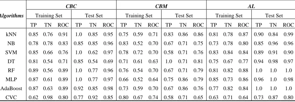
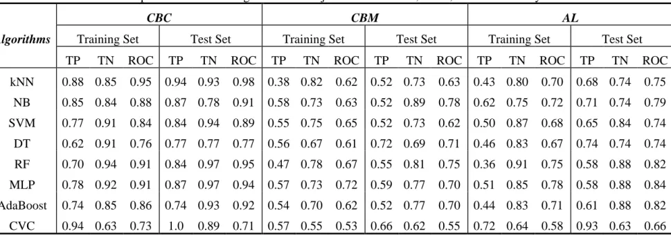
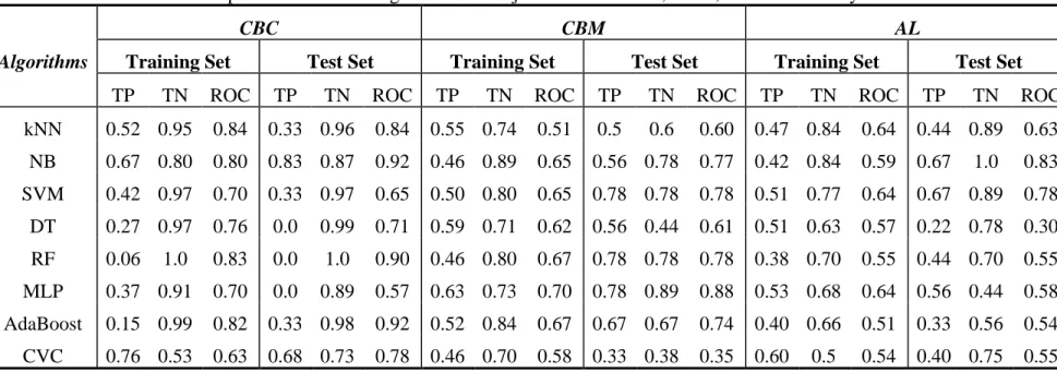
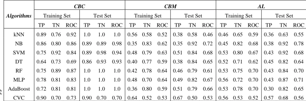
hERG Actives (A) vs. Inactives (I)………...………..……..……....60 3.8a Performance comparison of WEKA algorithms in conjunction with CBC, CBM,
and AL for study of hERG Blockers (B) vs. Activators (A)..………..……....63 3.8b Performance comparison of WEKA algorithms in conjunction with CBC, CBM, and
AL for study of hERG Blockers (B) vs. Inactives (I)..………..….………..……....64 3.8c Performance comparison of WEKA algorithms in conjunction with CBC, CBM, and AL for study of hERG Activators (A) vs. Inactives (I)..………..………65 3.8d Performance comparison of WEKA algorithms in conjunction with CBC, CBM, and
xi
3.9 Significant frequent descriptors that discriminate hERG Blockers (B) from
Activators (A)………....70 3.10 Significant frequent descriptors that discriminate hERG Blockers (B) from
Inactives (I)………...75 3.11 Significant frequent descriptors that discriminate hERG Activators (A) from the Inactives (I)………...80 3.12 Significant frequent descriptors that discriminate hERG Actives (A) from
Inactives (I) ………...85 4.1 Statistics of working datasets in mutagenicity and carcinogenicity of compounds..101
4.2 Performance of kNN QSAR classification studies for Mutagenicity modeling (mutagens vs. non-mutagens)…..………..…...………..…………102 4.3 Performance of kNN QSAR classification studies for Carcinogenicity modeling
(carcinogens vs. non-carcinogens) ………...………...…...…105 4.4 Performance of kNN QSAR classification studies for Carcinogenicity models
(genotoxic vs. non-genotoxic carcinogens)…...………..……...106 4.5 Performance of kNN QSAR classification studies for Epigenicity modeling I (genotoxic carcinogens vs. non-genotoxic carcinogens)………….………...……107 4.6 Performance of kNN QSAR classification studies for Epigenicity modeling II (genotoxic carcinogens vs. non-genotoxic non-carcinogens)...….………..……...109 4.7 Performance of kNN QSAR classification studies for Genotoxic Carcinogenicity
Modeling I(genotoxic carcinogens vs. genotoxic non-carcinogens)……...110 4.8 Performance of kNN QSAR classification studies for Genotoxic Carcinogenicity
Modeling II(genotoxic non-carcinogens vs. non-genotoxic non-carcinogens)….113 4.9 Performance of kNN QSAR classification studies for Mutagenicity, Carcinogenicity,
False Negatives and False Positives …..………..………..…..…..124 4.10a Comparative study of Lazar and kNN QSAR on prediction of mutagenicity for the
xii
4.11b Carcinogenicity structural alerts identified using Leadscope …………....…….130 4.12a Mutagenicity structural alerts identified by frequent descriptor analysis………132 4.12b Structural features that not induce carcinogenicity or mutagenicity identified by Frequent descriptor analysis....…….………..…….136 4.13 kNN QSAR models for mutagenicity and carcinogenicity showed high classifi-cation accuracy for external validation set ...………...156 4.S.1 Summary of kNN QSAR Modeling Result …..………...……..……….….163
4.S.2 Comparative study of Lazar and kNN QSAR for external evaluation set of 70 compounds………..……….165
xiii
LIST OF FIGURES
Figure
1.1 Principal components analysis (PCA) of hERG dataset showed outliers, class imbalance & overlap and small disjuncts ……….10 1.2 Frame work of imbalanced dataset classifier design that integrated data character-istics analysis and adapted to knowledge discovery & application needs……….13 2.1 Algorithm of Class Boundary Cleaning (CBC)………..…..………….26 2.2 Algorithm of Class Boundary Mining (CBM).……….……….27 2.3 Algorithm of Active Learning (AL).………..…….……….…….28 3.1 Principal components analysis (PCA) of hERG dataset showed outliers, class
imbalance & overlap and small disjuncts ………..………...…....46 3.2 Illustration of some algorithms developed in this work: Class Boundary Cleaning
(CBC), Class Boundary Mining (CBM) and Active Learning (AL)……….49 3.3 Structural features that discriminate hERG Blockers from Activators and suggest
options for lead optimization………..………...73 3.4 Structural features that discriminate hERG Blockers from Inactives and suggest
options for lead optimization………..………...79 3.5 Structural features that discriminate hERG Activators from Inactives and suggest
options for lead optimization………..………...……....83 3.6 Structural features that discriminate hERG Actives from Inactives and suggest
options for lead optimization…...…………...……….……...87 4.1 Toxicophores (promoting features) and toxicophobes (demoting features) for
xiv
genotoxic non-carcinogens by name, confidence, and P value..………...119 4.4 Significant descriptors detected by descriptor profiling.………..…...……..142 4.5a Significant descriptors profiling for mutagenicity.…………..………..…144 4.5b Confidence and P-Values of frequent descriptor for mutagenicity..……...…..…144 4.6a Frequent descriptor profiling for carcinogenicity….……...………..…..…..……146 4.6b Frequent descriptor profiling for carcinogenicity.…..……….…..…146 4.7a Frequent descriptor profiling for false negatives (non-genotoxic carcinogens)...148 4.7b Frequent descriptor profiling for false negatives (non-genotoxic carcinogens)...149 4.8a Frequent descriptor profiling for false positives (genotoxic non-carcinogens).…150 4.8b Top frequent descriptors and corresponding confidence and support to false positive
xv
ABBREVIATIONS
AD Applicability Domain AL Active Learning
CBC Class Boundary Cleaning CBM Class Boundary Mining
CPDB Berkeley Carcinogenic Potency Database CSL Cost Sensitive Learning
CVC Classification via Clustering
DSSTox Distributed Structure-Searchable Toxicity hERG human ether-a-go-go-related Gene kNN k Nearest Neighbors
Lazar lazy Structure-Activity Relationship LQTS long QT syndrome
MLP Multilayer Perceptron
NTP National Toxicology Program
QSAR Quantitative Structure-Activity Relationship SVM Support Vector Machine
SQTS Short QT Syndrome
EPA Environmental Protection Agency
CHAPTER I
INTRODUCTION Introduction of Imbalanced Dataset Mining
A dataset is imbalanced if at least one of the classes is represented by a significantly smaller number of instances, observations, examples or cases than others (Japkowicz, 2002; Abe, Naoki et al, 2003, Ertekin et al, 2007). Mining an imbalanced data set is a nontrivial issue. It has extensive applications in numerous fields that are essential for human life, for instance, rare disease or mutation diagnosis, credit card or insurance fraud detection (Fawcett and Provost, 1997), insurance risk modeling (Pednault, Rosen et al, 2000), airline no-show prediction (Lawrence, Hong et al, 2003), targeted marketing (Zadrozny & Elkan, 2001), intrusion detection and virtual high-throughput screening (HTS) in drug discovery. In the literature, the problem of imbalance is also known as dealing with rare cases or skewed data (Visa, 2005).
2
2005). With regard to algorithm design, (i) standard machine learning algorithms are designed to maximize overall accuracy while minimizing overall error rate; (ii) many standard classification algorithms assume even distribution, while class distributions in whole datasets, training, or test sets are not necessarily the same (Provost, 00; Weiss et al, 2001); (iii) misclassification costs for different classes are different, and may be unknown at learning time (Visa, et al, 2005). From the perspective of performance evaluation, overall prediction accuracy (the ratio of correctly classified instances over total number of instances in the dataset) might be inadequate because class distributions and misclassification costs are rarely uniform (Provost & Fawcett, 1997); and the use of such measures might lead to misleading conclusions. Accuracy or error rate assumes equal misclassification costs (Fawcett & Provost, 1997; Kubat, et al, 1997), which are not true in an imbalanced dataset. Evaluation metrics that take imbalance into account can improve classifier searching and selection (Weiss, 2004). Alternative measurements include ROC analysis*
*
ROC analysis: receiver operating chacteristic analysis, which can access trade off between precision and recall; AUC: Area under the ROC curve (AUC), which is not biased against the minority class; Precision: which is the percentage of times the predictions associated with the rule(s) are correct; Recall: is the percentage of all examples belonging to X that are covered by these rule(s); Geometric mean: the square root of precision times recall, reaching high value only if both precision and recall are high and in equilibrium; F-measure: parameterized weighted harmonic mean which can be adjusted to specify the relative importance of precision vs. recall; Precision Recall Break Even Point (PRBEP): the accuracy of positive class (smaller class) at the threshold where precision equals recall, it is another commonly used performance metric for imbalanced data classification; Matthews Correlation Coefficient (MCC): a measure of the quality of binary classifications, it is generally regarded as one of the best measures since it takes into account true and false positives and negatives, and can be used even if the classes are of very different sizes. , AUC, precision,
(
TP FP)(
TP FN)(
TN FP)(
TN FN)
FN FP TN TP MCC + + + + × − ×= , where TP is the number of true
3
recall, geometric mean, F-measure, Precision Recall Break Even Point (PRBEP) (Visa, 2005; Elkan, 2003; Ertekin et al, 2007), Matthews Correlation Coefficient (Matthews, 1975).
Numerous algorithms have been developed for mining imbalanced datasets (Table 1.1). Depending on where imbalance is handled, current algorithms fall into two main categories: re-sampling or re-balancing methods, which correct class imbalance at data level; and cost sensitive learning, which deals with imbalance at algorithm level (Abe, 2003; Chawla, 2003; Weiss, 2004).
4
4
Table 1.1: Survey of current algorithms for imbalanced dataset mining.
Category Methods Algorithms References Pros Cons
Data Level
Over Sampling SMOTE
Cluster-based resampling
Ling et al, 1998 Chawla et al, 2002
Jo et al, 2004
Effective in correct class imbalance Probability localized
Computational Cost↑ Over-fitting Risk↑ No information gain
Down Sampling
Random down-sampling Kubat et al, 1997 Japkowicz, 2001
Effective in correct class imbalance Probability localized Lost information Active Learning Adaptive Sampling Importance Sampling Selective Learning Query Learning Abe, 2003 Iyengar et al, 2000 Breiman et al, 1999
Ertekin et al, 2007 Provost, 1997
More efficient No information lost No increase of comp. cost
Algorithm Level Imbalance Insensitive Recursive Partition SVM Japkowicz, 2002 Visa et al, 2003
Insensitive to class imbalance Imbalance ratio limitation Cost Sensitive Learning Cost Penalty Decision Threshold Moving Weiss, 2007 Zadrozny et al, 2001
Pazzani et al, 1994 Kubat et al, 1998
Do well in big set Effective than random
sampling
5
of improving the classification accuracy (Iyengar, et al, 2000); Selective sampling uses only a small subset of labeled data for learning given a large number of (possibly unlabeled) data; Importance sampling concentrates on the examples near the classification boundaries. (Breiman, 1999) emphasized that Importance sampling pays off in terms of reduced generalization error, and it is better than query by bagging empirically.
Although resampling methods are popular because they are straightforward in correcting class imbalance, they have known drawbacks: 1) random over/up-sampling increases the training set size, computational cost and risk of over-fitting without any information gain, by adding exact copies of the smaller class examples (Provost 2000; Chawla, et al, 2002; Dummond, et al, 2003; Visa, 2005); 2) random down/under-sampling may suffer information loss by discarding potentially useful data (Japkowicz, 2001), thus it may degrade rather than improve classifier performance; 3) best class distribution is usually
unknown and needs to be investigated (Chan & Stolfo, 1998; Estabrooks & Japkowicz, 2004) prior to the subset generation; (Weiss & Provost 2003) showed that neither a balanced distribution nor the natural distribution is necessarily best for the learning task. 4) controversial results imply that inappropriate class ratio or other issues may involved. It has been reported that up-sampling or down-sampling solved the "problem" of imbalanced data sets in some studies, but didn’t help at all for other studies (Provost, 2001; Dummond et al, 2003; Kubat et al, 1997). Possible reasons are: the corrected class ratio after re-sampling is not appropriate for the dataset; other data structure features that degraded classifier’s performance have not been detected nor handled.
6
and Abe, ICML’00). In active learning, learners actively select each individual instance to train rather than take class distribution as given. While this principle of active learning (Provost, 2000) remains that same, the implementation of active learning varies. For example, Zheng used minimum number of compounds but kept the maximum diversity of the bigger class when balancing the two classes (Zheng et al, 2002); Kubat only removed majority class examples that are redundant, or bordering on minority class examples, which may be noise (Kubat et al, 1997). In many formal problems, active learning is provably more powerful than passive learning from randomly given examples (Cohn, 1994).
7
insensitive to class imbalance (but to a certain extent) such as recursive partitioning, or SVM. Japkowicz showed that their SVM implementation is not sensitive to class imbalances up to imbalance ratio of 1/16 (Japkowicz & Stephen, 2002). The sensitivity of recursive partitioning to class imbalance increases with the domain complexity and the degree of imbalance, but decreases with training set size (Japkowicz et al, 2002).
Right issues It is often assumed that class imbalance is responsible for significant loss of performance in standard classifiers; and all aforementioned algorithms focus on correct class imbalance directly or indirectly. However, Weiss and Provost demonstrated that neither a balanced distribution nor the natural distribution is the best for the learning task (Weiss & Provost, 2003). Japkowicz showed that the classifier’s performance for imbalanced data set related to three factors: concept complexity, training set size and degree of the imbalance (Japkowicz et al, 2000, 2002, 2003). They found that linearly separable domains are not sensitive to imbalance independently of the training size; as the degree of concept complexity increases, so does the system’s sensitivity to imbalance; with very large training data, the imbalance does not hinder the classifier’s performance too much. They concluded that class imbalance is a relative problem depending on both the complexity of the concept represented by the data and the overall size of the training set; class imbalance does not directly cause deterioration of classifier performance; the small disjuncts created by the class imbalance in highly complex and small-sized domains do. Moreover, Japkowicz indicated that his study did not cover all the characteristics a data domain may have (Japkowicz & Stephen, 2002).
8
other domain features that may hinder the performance of the classifiers. (Prati et al, 2004) demonstrated that the problem is not directly caused by class imbalances but the degree of overlap among classes. (Garcia et al, 2006) demonstrated that imbalance by itself will not strongly affect the classifier’s performance; performance deteriorates greatly when overlap increases. (Visa & Ralescu, 2003, 2004) showed that the overlap affects the fuzzy based classifier more than the imbalance; and the fuzzy classifier is affected by the imbalance only when data are of high complexity and small size, in which case the true problem is the lack of information, rather than imbalance ratio. (Weiss 2003) and (Jo & Japkowicz 2004) identified small disjuncts (subclusters in the minority class) as another hurdle in the classification of imbalanced datasets due to being poorly represented in the training set. (Weiss, 2004; Visa, 2005) elucidated that the following data chacteristics can all degrade classifier performance: improper evaluation metrics, lack of data (absolute or relative rarity), data fragmentation, noise and inappropriate inductive bias, which is the set of assumptions that the learner uses to predict outputs given inputs that it has not encountered (Mitchell, 1980). Therefore, it is not surprising to see an algorithm that only corrects class imbalance succeed in certain cases but fail in others (Provost, 2001; Dummond et al, 2003; Kubat et al, 1997). (Japkowicz, 2003) suggested that an algorithm should consider all fundamental domain characteristics that degrade classification, which necessitates carrying out exploratory data analysis and visualization before classifier design.
9
majority class; most of current algorithms deal with the pattern of minority class only, while overlooking the consequence of overlap between classes (Garcia, et al, 2006). However, real-world imbalanced datasets usually have unique characteristics: 1) the status of positive/minority or negative/majority class might not be fixed. For instances, in current hERG liability dataset, hERG blockers are the majority class comparing with hERG activators, but the minority class relative to inactives; 2) misclassification cost for the majority class can be very high as well. In this hERG liability study, both blockers and activators can cause fatal arrhythmia, but by different mechanisms; misclassification cost of either is forbiddingly high. However, each of them can be a potential cure for familiar SQTS or LQTS (Raschi et al, 2008), respectively. Therefore, for the sake of drug safety or therapeutic efficacy, we need to predict each and every class accurately; for the purpose of drug discovery and lead optimization, we need to discover structural features that can be used to tune out unwanted toxicity in lead compounds. However, current algorithms tailored to prediction accuracy of the minority class only are not sufficient for either of the purposes. Thus, beyond prediction accuracy, classifiers design shall adapt to data mining needs to maximize knowledge discovery and application.
10
compounds are structurally similar to each other but have different activities. The fine differences in structures between these compounds should explain the difference in their activities, and hence can be used to guide drug optimization – tuning out undesired toxicity without compromising the primary therapeutic efficacy. To find answer for this question, we need a new algorithm that mining data at class boundary; current algorithms that tailored to
improving prediction accuracy of the minority class only are not suitable.
Overview of Chapter II Methodology
Our central hypothesis is that in addition to class imbalance, other data domain characteristics such as class overlap (Figure 1.1), small disjuncts or clusters, and outliers all can contribute to deterioration of classifier performance. The only way to detect all those hidden characteristics is to do exploratory data analysis and data visualization. Problems detected within the data should be used as guidance for classifier selection and classifier
a b
11
design. On the other hand, classifier design shall meet the ultimate goal of data mining – knowledge discovery and application. Unmet needs in drug discovery, such as lead optimization by tuning out hERG liability, require development of new algorithms. Keeping data structure and data mining needs in mind, to improve the performance of classifiers and knowledge discovery, we designed classifiers as follows:
Class Boundary Cleaning (CBC)
The method is designed toclean up class overlap as well as reducing class imbalance. This is done by identifying compounds from the majority class that are within a certain distance of the minority class in high dimensional descriptor space, then removing them temporarily from the model building. The optimal distance can be defined by sampling different distance thresholds and consequent model building. Since the cleaning is only executed for the majority class, it reduces the class imbalance at the same time.
Class Boundary Mining (CBM)
The methodis developed tosearche, define, optimize and learn from class boundary – the region where compounds from different classes are structurally similar and geometrically close to each other, yet have different activities. By sampling different distance thresholds, different compounds are pooled and learned; ideally the fine structural differences between two classes of compounds should be picked up by distinguishing models; and that shall give us clues about how to reduce or remove undesired activity of a drug.
Active Learning (AL)
12
to class boundary. The difference between CBM and AL is that AL keeps all the rare cases, thus using the information of rare instances in a somewhat better way.
Cost Sensitive Learning (CSL)
The method assigns a greater cost to each case of misclassification of the minority class than those of the majority class. This approach improves performance with respect to the positive (minority) class (Weiss, 2004). It is done by including decision thresholds, weights for different classes, and misclassification costs into standard QSAR procedures, in our case, kNN QSAR category algorithm that developed in our laboratory. Ideally, these parameters should be optimized, i.e. the values should be found which give models with highest predictivity.
Outlier Removal (OR)
The method is designed to identify and remove outliers that may degrade performance of classifier. It is done by searching compounds in the dataset that have no nearest neighbors within different distance thresholds (i.e. outliers are defined by a distance threshold).
Resampling
The method is designed to correct class imbalance, by resampling the original training dataset to create more balanced classes. This is done either by oversampling the minority class or under-sampling the majority class until the classes are approximately equally represented.
13
of classifiers targeting domain characteristics detected in the first step; (iii) design of classifiers that incorporate data mining goals. Without data domain diagnosis, it will be impossible to find out hidden detrimental domain characteristics other than class imbalance; using algorithms that correct class imbalance only will generate mixed results – which work in certain cases but fail in others as reported in literature (Provost, 2001; Dummond et al, 2003; Kubat et al, 1997).
For comparison, we studied the performance of in-house kNN QSAR classification algorithm with and without combination with aforementioned algorithms; we also studied the performance of WEKA algorithms before and after data preprocessing with the algorithms we developed.
Overview of Chapter III Pattern Classification and Knowledge Discovery in QSAR Studies of Imbalanced Data Set of hERG Liability
Y Randomization Combi-QSAR Modeling Activity Prediction Only accept models have a
CCR > 0.6
Validated Predictive Models with High Internal
& External Accuracy
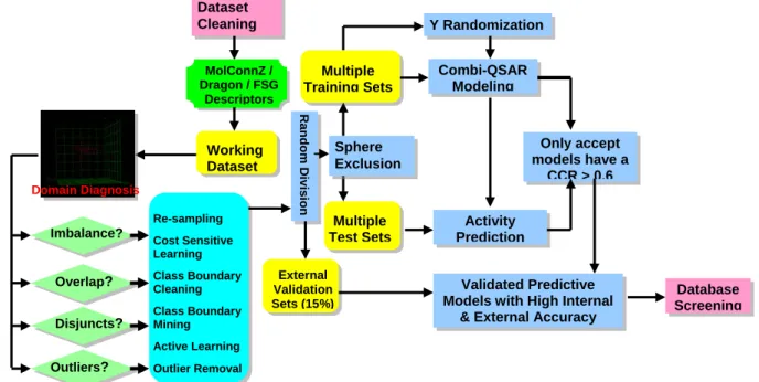
Database Screening Working Dataset Multiple Test Sets External Validation Sets (15%) Multiple Training Sets R a ndom D iv is ion Sphere Exclusion Dataset Cleaning MolConnZ / Dragon / FSG Descriptors Domain Diagnosis Imbalance? Overlap? Disjuncts? Outliers?
Figure 1.2. Framework of imbalanced dataset classifier design that integrated data chacteristics analysis (domain diagnosis) and adapted to knowledge discovery and application needs.
14
The human ether-a-go-go related gene (hERG) K+ channel can be both antitarget and target in drug discovery. As antitarget, drug induced blockade of hERG K+ channel can cause QT prolongation, TdP and fatal arrhythmia, thus it is important to screen out hERG channel blockers at early stage of drug discovery. As target, hERG blockers can be potential class III anti-arrhythmics, or possible therapeutics for congenital short QT syndrome (Raschi et al, 2008). hERG openers shorten QTS, and can work as potential therapeutics for congenital LQTS (Fermini and Fossa 2003). On the other hand, the inactive compounds, especially those located at class boundary, may contain valuable chemical information that can be used to tune out hERG liability from lead compounds for other non-cardio therapeutics at the stage of drug optimization. Therefore, all three classes in this particular dataset are very important in their own terms to drug discovery.
15
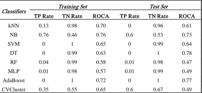
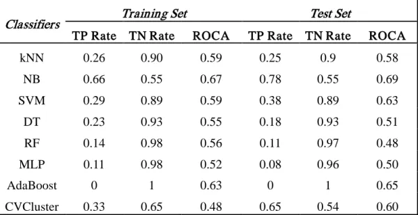
Bayesian, Support Vector Machine (SVM), Decision Tree, Random Forest, Multilayer Perceptron (MLP), AdaBoost, and Classification Via Clustering (CVC), etc. As further comparison, we performed the same studies using those WEKA algorithms combined with CBC, CBM and AL, the results showed that CBC, CBM and AL can improve WEKA classifier’s performance.
We performed frequent descriptor analysis of those highly predictive models, and discovered chemical structural patterns that either promote or demote hERG liability with different levels of confidence. Those promoting or demoting structural features can be used to alert or tune out hERG liability, respectively. In addition to drug screening or lead optimization, that knowledge can extend application of hERG liability prediction in governmental regulatory work.
Overview of Chapter IV Classification and Knowledge Discovery for Mutagenicity
andCarcinogenicity in Carcinogenic Potency Database (CPDB)
Accurate prediction of the chemical carcinogenicity is a scientific issue of unquestionable importance. Cancer is the most feared disease in the modern world, the second largest cause of death. It affects one person in three at all ages (American Cancer Society, December 2007), and costs hundreds of billions of dollars in medical expenses each year. Accurate prediction of carcinogenicity potential of compounds is crucial for the prevention of chemically-induced cancer.
16
chromosome aberration (CA), sister chromatid exchanges (SCEs) etc, are fast and cost-effective but currently insufficient to accurately and reliably predict the outcome of long-term carcinogenicity studies (Kirkland et al, 2008; Ashyby, 1993). SAR methods overall produced a higher concordance frequency and a lower percentage of false negatives than the overall genetic toxicity test methods (Ashyby, 1988). Structural alerts (SAs) qualitatively point to the potential of a compound to induce cancer by direct DNA damage, but not by epigenetic mechanisms. Compared with SAs, QSAR models are preferred in virtual screening as more powerful, efficient and reproducible. However, for in silico toxicity prediction software such as MCASE, DEREK, OncoLogic and TOPKAT, HazardExpert etc (Benigni, 1997; Ashyby and Tennant, 1991), high false negative rate and false positive rate have always been problems. Many studies have been carried out to reduce false positive and false negative rates, such as threshold moving to correct statistical prediction errors. Consequently, sensitivity was improved at the price of specificity or vice versa. Very little systematic research has been done to elucidate the chemical mechanistic information behind the phenomena, and to differentiate false negatives and false positives from genotoxic carcinogens better.
17
chemicals (salts and metals). Chiral compounds were removed as well. We took into account both mutagenicity and carcinogenicity simultaneously, and created working sets for different studies shown in Table 4.1.
Working sets have different levels of class imbalance. They will be a good source for cross-references. The models will be examples of how class imbalance affects the performance of classifiers. We expect models built and chemical patterns found will be useful for reducing the risk of hidden hazards, animals sacrificed for toxicity tests, and undue concerns as well.
Overview of Chapter V Summary and Future Studies
In the last chapter of this dissertation, I summarized the novel methodology I developed for the important, challenging issue in the data mining field – imbalanced dataset classification, plus its potential significant application in drug discovery and development. Two supporting research projects were also reviewed for the results, knowledge discovered and potential application, and future studies.
CHAPTER II
METHODOLOGY
Novel algorithms were developed based on core technology – kNN QSAR classification that was developed in the lab – to improve the performance of classifiers for imbalanced dataset and improve knowledge discovery. These new algorithms outperformed WEKA algorithms in mining the imbalanced hERG liability dataset. What’s more, the new algorithm demonstrated unique edge in discovering chermical patterns for lead optimization during drug discovery. In this chapter, the background information about QSAR will be briefly introduced first, and then methodology developed will be presented, followed by explaining WEKA algorithms in comparison.
Background Information of QSAR
QSAR, which stands for Quantitative Structure-Activity Relationship, is a statistic learning methodology of searching, optimizing and validating the best possible mathematic equations that quantitatively correlate a set of defined biological or chemical activities, such as inhibition or activation of hERG K+ channel, being mutagenic or carcinogenic or not, etc. QSAR's most general mathematical form is:
19
Once established, the mathematical expression can be used to predict the biological response of other similar chemical structures.
As its name and equation suggest, QSAR has three core components: chemical structures, activity and the mathematical relationship between the two. Chemical structures were quantitatively expressed by descriptors, such as functional groups, as well as their physicochemical properties etc. We will review QSAR methodology by structural descriptors first, and then the development and validation of the mathematic relationship.
Descr iptor s Used
There are many types of chemical structural descriptors. Three types of descriptors used in this dissertation project are listed as follows:
Molconn-Z Chemical Descriptors:
20
in multidimensional descriptor space as well as in feature selection during kNN model building procedure (see below).
Dr agon Descr iptor s
A set of 843 theoretical molecular descriptors was computed using DRAGON software (Talete s.r.l. Dragon, 2007). The descriptors were generated from the SMILES strings available for each compound. The descriptors includ the following types: 0D constitutional (atom and group counts); 1D functional groups; 1D atom centered fragments; 2D topological descriptors; 2D walk and path counts; 2D autocorrelations; 2D connectivity indices; 2D information indices; 2D topological charge indices; 2D Eigenvalue-based indices; 2D edge adjacency indices; 2D Burden eigenvalues and molecular properties. Dragon descriptors were range-scaled. Variables which had the same value for all compounds were deleted. If two descriptors were at least 98% correlated one of them was deleted. The final sets used in QSAR studies included about 350 descriptors. The definition of these descriptors and related literature references are reported elsewhere (Todeschini et al, 2007).
Fr equent Subgraph Descr iptor s
21
activity, or the toxicophores for the toxicity, of molecules in different datasets. Compared to descriptors with fixed types and sizes of built-in functional group library in commercial software, descriptors generated by this method is more dataset specific, and more likely to catch novel structural features that are unique for particular activity.
kNN QSAR Methodology
Model Development and Validation
Training, Test and External evaluation set After preprocessing, the datasets were randomly divided into modeling and external evaluation sets which included about 85% and 15% of compounds of entire datasets, respectively. Modeling sets were further divided into multiple training and test sets of different sizes (see below). Training sets were used for building QSAR models. Test sets were used for validation of QSAR models. External evaluation sets were used for additional validation of QSAR models which had high predictive accuracy of the training sets in the leave-one-out cross-validation procedure (see below) and the test sets. Consensus prediction was applied for external validation. Thus, external evaluation sets were used as an objective evaluation of prediction of compounds not included in the original dataset. In validation of QSAR models using test and external evaluation sets, predictions were made for compounds within rigorously defined applicability domains (AD). High prediction accuracy for external evaluation sets would confirm the predictive power of QSAR models and their applicability for classification of other compounds.
22
the calculation of the distance matrix D between points that represent compounds in the descriptor space. Let Dmin and Dmax be the minimum and maximum elements of D, respectively. N probe sphere radii are defined by the following formulas. Rmin = R1 = Dmin,
Rmax = RN = Dmax/4, Ri = R1 + (i-1)*(RN-R1)/(N-1), where i = 2, ..., N-1. Each probe sphere
23
algorithm, the composition of training and test sets is different for different original dataset divisions.
kNN QSAR Method The kNN QSAR method employs the kNN pattern recognition principle and a variable selection procedure. Initially, a subset of nvar (number of selected variables) descriptors is selected randomly. Then the selected subset of descriptors is modified based on the values of prediction accuracy (see below) in the leave-one-out cross-validation procedure, in which each compound in turn is eliminated from the training set and its biological activity is predicted as the weighted-by-distance average activity of k most similar molecules (k=1 to 5) in the selected nvar descriptor subspace. (The molecular dissimilarity was characterized by the Euclidean distance between compounds in the nvar-subspace of the multidimensional descriptor space.) In general, the Euclidean distances in the descriptor space between a compound and each of its k nearest neighbors (k>1) are not the same. Thus, the neighbor with the smaller distance from a compound was given a higher weight in calculating the predicted activity as follows (Eq. 1 & 2):
∑
= − = k j ij ij ij d d w 1 ' '1 [1]
∑
∑
= = = k j ij k j ij j i w w y y 1 1ˆ [2]
where dij is the Euclidean distance between compound i and its k-th nearest neighbor; wij is the weight for every individual nearest neighbor; yi is the observed activity value for nearest neighbor i; and ŷi is the predicted activity value of compound i. If k=1, yˆi = y1. In case of
24
annealing with the Metropolis-like acceptance criteria is used to optimize the variable selection. The optimization criterion (prediction accuracy), or correct classification rate (CCR) is defined as:
+ = totalcorr totalcorr
N N N N CCR 1 1 0 0 5 .
0 [3]
where 0 and 1 are class numbers (e.g., non-carcinogenic and carcinogenic, Nicorr and Nitotal are the number of correctly predicted and total number of compounds of class i. The ratio
total i corr i N N
is also called specificity and sensitivity, respectively, for class i=0 and i=1. For truly
predictive models, both sensitivity and specificity should be close to one. For compounds not included in the training set prediction is made using the same formulas [1] and [2], and nearest neighbors are taken from the training set. For all the training, test and external evaluation sets, CCR are used as criteria of prediction accuracy.
In summary, the kNN-QSAR algorithm generates both an optimal k value and an optimal nvar subset of descriptors, that afford a QSAR model with the highest training set model accuracy as estimated by the CCR value. Further details of the kNN method implementation, including the description of the simulated annealing procedure used for stochastic sampling of the descriptor space, are given in our previous publications (Roberts, Myatt et al, 2000; Shen, Xiao et al, 2003; Ng, Xiao et al, 2004).
25
threshold) should be introduced to avoid making predictions for compounds that differ substantially from the training set molecules. Suppose that a model includes M descriptors, i.e. each compound can be represented by a point in the M-dimensional descriptor space with the coordinates Xi1, Xi2, ..., XiM, where Xis are the values of individual descriptors. The molecular dissimilarity between any two molecules was characterized by the Euclidean distance between their representative points. The Euclidean distance dij between two points i and j (which correspond to compounds i and j) in M-dimensional space is calculated as follows (Eq. 4):
(
)
∑
=
−
= M
k
jk ik
ij X X
d
1
2
[4]
Compounds with the smallest distance between one another are considered to have the highest similarity. Let y and σ be the mean and standard deviation of distances between compounds and their K nearest neighbors in the training set, then the applicability domain threshold, ADT, is defined as follows (Eq. 5):
ADT = y + Zσ [5]
Here, Z is an arbitrary parameter called Z-cutoff. Based on previous studies (Shen, LeTiran et al, 2002), we set the default value of this parameter to 0.5, but other values such as 1.0 or 1.5 can be used as well. Thus, if the distance of the external compound from the closest of its k nearest neighbors in the training set exceeds this threshold, the prediction is not done.
26
Algorithm 1:Class Boundary Cleaning Input: S (data set with n instances)
Parameters: Z (applicability domain)
Output: Az (clean data set)
S1 = DataPartition S (class 1)
S0 = DataPartition S (class 0)
S01 = SimilarityMatrix_EuclidianDistance (S0, S1)
If size(S0)> size(S1)
for Z = 0 to 3.0 do
A01 = RemoveInstancesSimilarToClass 1 AtThreshold Z (S0 – S01)
Az = A10 U A01
Z += 0.5 end for
return Az
# Az is ready to input standard kNN QSAR Classification workflow end if
Figure 2.1: Algorithm of Class Boundary Cleaning (CBC).
than the models built using the training set with real activities, or the total number of "acceptable" models based on the randomized training set satisfying the same cutoff criteria (CCR (train) > 0.7 and CCR (test) > 0.7) should be much lower (at least one order) than those based on the training set with real activities. If this condition is not satisfied, models built with real activities for this training set are not reliable and should be discarded. This test was applied to all data divisions considered in this study.
Methodology Developed
Class Boundary Cleaning (CBC) This method is designed to reduce class overlap (Fig. 2.1). Cleaning could be done in two classes. To avoid worsening class imbalance, it was performed for the majority class only, i.e. com-pounds from the majority class that are close
27
Algorithm 2:Class Boundary Mining Input: S (data set with n instances)
Parameters: Z (applicability domain)
Output: A (clean data set)
S1 = DataPartition S (class 1)
S0 = DataPartition S (class 0)
S10 = SimilarityMatrix_EuclidianDistance (class 1 to class 0)
S01 = SimilarityMatrix EuclidianDistance (class 0 to class 1)
for Z = 0 to 3.0 do
A10 = CollectInstancesSimilarToClass 0 AtThreshold Z (S1 – S10)
A01 = CollectInstancesSimilarToClass 1 AtThreshold Z (S0 – S01)
Az = DataFusion (A10+A01)
Z += 0.5 end for
return Az
feed Az to standard kNN QSAR Classification workflow
Figure 2.2 Algorithm of Class Boundary Mining (CBM).
were removed, class imbalance was alleviated along with the class overlap, and the effect increased with the distance threshold.
Class Boundary Mining (CBM) This method is developed to search, define, optimize and learn from the class boundary – the region where compounds from different classes are structurally similar and geometrically close to each other, yet have different activities labels (Fig. 2.2). By sampling different distance thresholds, different compounds are pooled and trained; ideally the fine structural differences between two classes of
28
Algorithm 3:Active Learning Input: S (data set with n instances)
Parameters: Z (applicability domain)
Output: A (clean data set)
S1 = DataPartition S (class 1)
S0 = DataPartition S (class 0)
if S0 > S1
S01 = SimilarityMatrix EuclidianDistance (class 0 to class 1)
for Z = 0 to 3.0 do
A01 = RemoveInstancesSimilarToClass 1 AtThreshold Z (S0 – S01)
Az = DataFusion (S1+A01)
Z += 0.5 end for
return Az
feed Az to standard kNN QSAR Classification workflow end if
Figure 2.3: Algorithm for Active Learning (AL).
Active Learning (AL) The main idea of active learning is to actively select training examples rather than passively taking input as given (Cohn, 1994). The principle of active learning is to reduce the number of training examples needed while maintaining the quality of resulting classifiers. AL is designed to enhance data mining efficiency, especially for the scenario where not every example is equally important or informative. (Breiman, 1999) demonstrated that in classification, concentrating on the examples near the classification boundaries pays off in terms of reduced generalization error. The paradigm of active learning falls into two major subfields: membership queries and selective sampling (Lindenbaum, 1999). In this study, Active Learning was implemented as Fig. 2.3 to select majority class objects that are close to the minority class boundary. Ideally this sampling step will correct class imbalance, reduce classification error without inducing information loss or
29
Cost Sensitive Learning (CSL) kNN QSAR To make the learning function of aforementioned kNN QSAR category method cost sensitive, we introduce decision threshold and misclassification penalty into evaluation metrics for imbalanced dataset classification as follows: ≤ ≤ ≤ ≤ = =
∑
∑
= = 1 , 1 0 , 0 1 1 i i k j ij k j ij j i y t t y w w y y [6] P N N w N N wCCRi = × + × tot −
1 Corr 1 1 tot 0 Corr 0
0 [7]
tot 1 Corr 1 tot 0 Corr 0 N N N N P
P= c⋅ − [8]
where yiis the predicted activity value of compound i; t is the decision threshold, instead of 0.5 for rounding to the closest integer; yi
is rounded to 0 if it is smaller than t, or 1 if it is higher; CCRi is correct classification rate for imbalanced dataset; wi is weight for class i;
tot i
N andNicorrare correctly predicted and total number for class i; P is misclassification penalty; Pc is misclassification penalty coefficient. Ideally, optimal parameters t, w0, w1 and Pc could be found that would be sensitive to high misclassification cost of the minority class
and enable equal or higher tot corr N N
0 0
and tot corr N N
1 1
despite high class ratio.
30
choice; 4) remove those compounds that have no neighbors within certain z cutoff thresholds, keeping the rest of compounds as the working set for the next step.
Inter-class Rare Instance Over-Sampling (RIOS_Inter) This method was done in a similar way as above, except that rather than removed those compounds with no neighbors at certain z cut-off, we simply duplicated those compounds.
Intra-class rare Instance Over-Sampling (RIOS_Intra) This method was also done in a similar way; just the first step was done within each class, and then duplicated the “loner” compounds either in both classes or only the minority class, respectively, depending on whether small clusters or class imbalance is the main concern of that particular dataset.
WEKA Softwar e and Algor ithms Used
WEKA stands for the Waikato Environment for Knowledge Analysis, which was developed at the University of Waikato in New Zealand. It was written in Java and distributed under the GNU Public License (Witten and Frank, 2005). It is a comprehensive software package that includes data pre-processing tools, machine learning algorithms and evaluation methods for data mining tasks. The algorithms can either be applied directly to a dataset or called from your own Java code. WEKA machine learning tools contains algorithms for classification, regression, clustering, association rules, and visualization. It is well-suited for comparing learning algorithms, as well as developing new machine learning schemes.
31
developed, as well as comparing performance of these algorithms before and after combining them with approaches we developed. Herein, we briefly introduce these algorithms and corresponding parameters used as follows.
IBk This algorithm is the WEKA implementation of K-nearest neighbors (kNN) classifier based on Aha and Kibler’s work on instance-based learning algorithms (Aha and Kibler, 1991). Optimal parameters we selected for this algorithm are: three nearest neighbors, inverse-distance-weighting, ten-fold cross-validation and linear nearest neighbor searching algorithm.
NaïveBayes This algorithm is WEKA implementation of Naive Bayes classifier using estimator classes based on John and Langley’s work (John and Langley, 1995). Numeric estimator precision values are chosen based on analysis of the training data. In this study, the following parameters are used for this algorithm: useKernelEstimator as true for using a kernel to estimate numeric attributes instead of using normal distribution; useSupervisedDiscretization as false for not using supervised discretization to convert numeric attributes to nominal ones.
32
J 48 This algorithm is the WEKA implementation of C4.5 decision tree based on work by Quinlan (Quinlan, 1993). The optimal parameters we selected for this algorithm are: use binary Splits on nominal attributes when building the trees; confidence Factor of 2.5 for pruning; the minimum number of instances per leaf as 2; counts at leaves are smoothed based on Laplace.
RandomF orest This algorithm is the WEKA implementation of a classifier for constructing a forest of random trees based on work of (Breiman, 2001). In this study, we used the following parameters: maxDepth as 0 for unlimited maximum depth of the trees; numFeatures as 50 for the number of attributes to be used in random selection; numTrees as 250 for the number of trees to be generated; seed as 10 for the random number seed to be used.
33
initialize the random number generator; Random numbers are used for setting the initial weights of the connections between nodes, and also for shuffling the training data; reset as true to allow the network to reset with a lower learning rate to restart training again if the network diverges from the answer; trainingTime as 500 epochs to train through; validationSetSize as 0 for the network to train for the specified number of epochs; validationThreshold as 20 to terminate validation testing when the validation set error is worse 20 times in a row before training is terminated.
AdaBoost AdaBoost stands for adaptive boosting. It is the WEKA implementation of Adaboost M1 method for boosting a nominal class classifier based on work of Freund and Schapire (Freund and Schapire, 1996). Only nominal class problems can be tackled by this method. It often dramatically improves the performance of a weak classifier, but sometimes over-fits. Parameters we optimized and set are: Decision Stump as classifier to use; numIterations as 100 iterations to perform; seed as 1 for random number generation; useResampling as false; weightThreshold as 100 for weight pruning.
34
belonging to each of the clusters. EM can decide how many clusters to create by cross validation, or you may specify a priori how many clusters to generate.
Toxicophor es and Toxicophobes Identification and Validation
Gener al Pr ocedur es The first step towards the identification of toxicophores or toxicophobes was generation of highly predictive models, followed by examination of the models with test sets and external validation sets; The second step is frequent descriptor analysis over the models that showed high prediction accuracy for the training, test and external validation sets; The third step is association rule learning of the significant structure feature/descriptors detected in step two. The support, confidence and p-value will show whether the structures were an interesting or significant (p < = 0.05) pattern that is capable of promoting (confidence > 0.5, toxicophores) or demoting (confidence < 0.5, toxicophobes) specific toxicity in the dataset.
Support The support suup(X) of a substructure (or toxicophore) is the percentage of compounds in the dataset D that contain this substructure.
D X count X
suup( )= ( )/ [9] Confidence The confidence of a substructure (or toxicophore) is the percentage of experimentally determined toxicants in the subset of compounds that contain this substructure
CHAPTER III
Pattern Classification and Knowledge Discovery in QSAR Studies of Imbalanced Data Set of hERG Liability
Intr oduction
36
Implication for drug design & current status of research Because of aforementioned inadvertent lethal toxicity, hERG K+ channel was mainly taken as an antitarget in drug development; current research on hERG liability prediction has overwhelmingly focused on screening out potential hERG blockers at the earliest stage of drug discovery (Fermini and Fossa 2003). However, the recent identification and functional characterization of hERG K+ channels, not only in the heart but also in several other tissues (e.g. neurons, smooth muscle and cancer cells), suggests that hERG can also be a possible target for antipsychotic, muscle atrophy, oncology and cardiology drugs (Witchel 2007; Raschi, Vasina et al, 2008). As hERG blockers, Class I antiarrhythmics can be promising therapeutics for short QT syndrome (SQTS) (Gaita, Giustetto et al, 2004; Milberg, Fleischer et al, 2007); Class III antiarrhythmics can prevent reentry arrhythmia and be second-line therapy for SQTS (Wolpert, Schimpf et al, 2005; Antzelevitch 2007). hERG activators shorten QT interval and can be potential new therapeutics in the treatment of delayed depolarization conditions, which may happen in patients with inherited and acquired LQTS (Zhou, Augelli-Szafran et al, 2005; Raschi, Vasina et al, 2008). Therefore, to make drug discovery process more safe, efficient and cost effective, it is important to distinguish and screen out potential hERG blockers and activators at early stage of drug discovery, if hERG is the primary therapeutic target. Otherwise, tuning-out hERG liability without compromising its primary therapeutic efficacy should be considered before throwing out a promising lead from drug discovery pipeline. For that purpose, sound and practical medicinal chemistry strategies are needed (Aronov 2006; Stansfeld, Gedeck et al, 2007; Judd, Souers et al, 2008; Lagrutta, Trepakova et al, 2008).
37
38
the membrane potential of cells. However, depolarization is not linearly correlated with current inhibition, and fluorescence artifacts of compounds can confound interpretation of results (Lagrutta, Trepakova et al, 2008). Thus the methods are prone to generate false-negative results with less potent inhibitors (Murphy, Palmer et al, 2006). Considering the pros and cons of experimental assessment of hERG inhibition, reliable, efficient and cost-effective in silico predictive tools are needed for the screening and optimization of drug candidates (Witchel, Hancox et al, 2003; Gavaghan, Arnby et al, 2007).
39
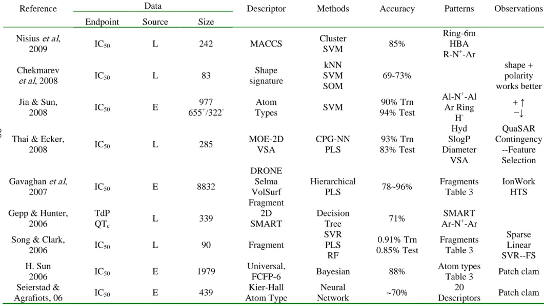
Table 3.1. Summary of current studies of in silico prediction of hERG liability.
Reference Data Descriptor Methods Accuracy Patterns Observations
Endpoint Source Size Nisius et al,
2009 IC50 L 242 MACCS
Cluster
SVM 85%
Ring-6m HBA R-N+-Ar Chekmarev
et al, 2008 IC50 L 83
Shape signature kNN SVM SOM 69-73% shape + polarity works better Jia & Sun,
2008 IC50 E
977 655+/322
-Atom
Types SVM
90% Trn 94% Test
Al-N+-Al Ar Ring
H-
+ ↑ −↓
Thai & Ecker,
2008 IC50 L 285
MOE-2D VSA CPG-NN PLS 93% Trn 83% Test Hyd SlogP Diameter VSA QuaSAR Contingency --Feature Selection Gavaghan et al,
2007 IC50 E 8832
DRONE Selma VolSurf Fragment
Hierarchical
PLS 78~96%
Fragments Table 3
IonWork HTS Gepp & Hunter,
2006
TdP QTc
L 339 2D
SMART
Decision
Tree 71%
SMART Ar-N+-Ar Song & Clark,
2006 IC50 L 90 Fragment
SVR PLS RF 0.91% Trn 0.85% Test Fragments Table 3 Sparse Linear SVR--FS H. Sun
2006 IC50 E 1979
Universal,
FCFP-6 Bayesian 88%
Atom types
Table 3 Patch clam Seierstad &
Agrafiots, 06 IC50 E 439
Kier-Hall Atom Type
Neural
Network ~70%
20
40
Reference Data Descriptor Methods Accuracy Patterns Observations
Endpoint Source Size
ISIS Keys Atom Pairs
EState MOE
Table 2
Dubus et al,
2006 IC50 E 203 2D MOE RP 81%
LogP, VSA SMR Ekins
et al, 06 IC50 L 99
Smart Mining® SOM Sammon RP 81-95% Hdy HBD S(=CH) S(>N-) AM Aronov
2006 IC50 E 194 MOE
Pharmacophore MOE 5pt: 70%~ 80% 6pt: 21%~44% Hyd, HBA ClogP Pharmaco -phores (2x5pt, 1x6pt) Neutral blocker; T623, S624 Partial fit is sufficient Cianchetta et al,
2005 IC50 E 882 GRIND
HQSAR PLS
r2=0.76 q2=0.72
N+--HBD HBA Hyd Charged & Neutral Blockers Aronov &
Goldman, 2004 IC50 E
414 85+/329-
Topology Pharmacophore
Pharmacophore
ensemble 82%
CLogP MR, pKa
Bains et al, 2004
IC50 L 124 Fragment
GA
EP 85-90%
2 Hyd 1 Ar 1 N+ Roche
et al, 2002 IC50 E 472
TSAR CATS VolSurf Dragon SOM PLS PCA NN 71% Blockers 93% Non- Blockers 2 motifs (1/0)
41
Reference Data Descriptor Methods Accuracy Patterns Observations
Endpoint Source Size
3D
Cio et al,2008 EC50 E 18
Homology MD Docking N+ Ar-G657/S624 Hyd~F656/T652 ECG g/kg?! C-State?
Farid et al, 2006 IC50 C 11 Homology
Docking
{N+ -F656/T652, Polar-S624,
HB}
KvAP (open) Rajamani et al,
2005 IC50 L 32
Homology LIE
RMSD=0.5 r2=0.82
∆vdw outweighs ∆ele Dual states KcsA (close) MthK(open) Pearlstein et al,
2003 IC50 E 32
Homology Docking CoMSiA
q2=0.57
Ar/Hyd-F656 N+-T652 Pore Diameter
Loop Depth
MthK (open) Cavali
et al, 02 IC50 L 31 CoMFA
r2=0.95 q2=0.77
2 Ar 1 3rd N
42
pharmacophore model can be both descriptive and predictive (Cavalli, Poluzzi et al, 2002; Ekins, Crumb et al, 2002; Pearlstein, Vaz et al, 2003; Aronov and Goldman, 2004; Bains, Basman et al, 2004; Peukert, Brendel et al, 2004; Sanguinetti and Mitcheson 2005; Aronov, 2006; Johnson, Yue et al, 2007; Leong 2007), thus it can have extensive applications to database screening. However, the application can be tricky: depending on the size and diversity of the dataset the pharmacophore is derived from, it could be too general for a huge, diverse dataset, or too specific for a small series of molecules; besides, considerable variation of pharmacophore features within or accross chemical series can be tolerated without significant reduction in potency of hERG blockade (Pearlstein, Vaz et al, 2003).
43
moeties based on a dataset of 339 compounds (Gepp and Hutter 2006). Cianchetta and Aronov independently built predictive models and found that hydrophobicity and hydrogen bond acceptors are critical pharmacophore features for neutral hERG blockers (Cianchetta, Li et al, 2005; Aronov 2006). Dubus and Aronov separately found that LogP and molecular refractivity are critical for decision tree models to be highly predictive (Aronov and Goldman 2004; Dubus, Ijjaali et al, 2006). However, the hERG liability screening used in the pharmaceutical industry can have positive rates as high as 60% (Zhou, Augelli-Szafran et al, 2005; Shah 2006), which implies that the false positive rate is high. This necessitates more accurate and reliable in silico methods.
Massive efforts have been made to elucidate molecular characteristics that indicate hERG blockade and use them to screen out blockers (Pearlstein, Vaz et al, 2003); only a few works have been published on eliminating hERG blockade or liability (Aronov 2008; Judd, Souers et al, 2008); even less research has been done on hERG activators. However, these in conjunction with the following questions deserve no less attention: what chemical characteristics of these two groups of compounds enable them to bind to the same target? what chemical characteristics decide them to have different activities? what chemical features can be modified to tune out hERG liability? Driven to tackle those interesting problems, we found these seemingly straightforward classification tasks have many challenging technique issues.
Drugs that induce hERG blockade are known for their diversity hERG K+ channel is known to be promiscuous – the binding ligands encompass diverse structural and