Efficient computation of discrete Voronoi diagram and homotopy-preserving simplified medial axis of a 3d polyhedron

(1)

Efficient Computation of Discrete Voronoi Diagram and

Homotopy-Preserving Simplified Medial Axis of a 3D

Polyhedron

by Avneesh Sud

A dissertation submitted to the faculty of the University of North Carolina at Chapel Hill in partial fulfillment of the requirements for the degree of Doctor of Philosophy in the Depart-ment of Computer Science.

Chapel Hill 2006

Approved by:

Dinesh Manocha, Advisor Ming C. Lin, Reader Mark Foskey, Reader

(2)

(3)

c 2006 Avneesh Sud

(4)

(5)

ABSTRACT

AVNEESH SUD: Efficient Computation of Discrete Voronoi Diagram and Homotopy-Preserving Simplified Medial Axis of a 3D Polyhedron.

(Under the direction of Dinesh Manocha.)

The Voronoi diagram is a fundamental geometric data structure and has been well studied in computational geometry and related areas. A Voronoi diagram defined using the Euclidean distance metric is also closely related to the Blum medial axis, a well known skeletal repre-sentation. Voronoi diagrams and medial axes have been shown useful for many 3D computa-tions and operacomputa-tions, including proximity queries, motion planning, mesh generation, finite element analysis, and shape analysis. However, their application to complex 3D polyhedral and deformable models has been limited. This is due to the difficulty of computing exact Voronoi diagrams in an efficient and reliable manner.

In this dissertation, we bridge this gap by presenting efficient algorithms to compute discrete Voronoi diagrams and simplified medial axes of 3D polyhedral models with geo-metric and topological guarantees. We apply these algorithms to complex 3D models and use them to perform interactive proximity queries, motion planning and skeletal computa-tions. We present three new results. First, we describe an algorithm to compute 3D distance fields of geometric models by using a linear factorization of Euclidean distance vectors. This formulation maps directly to the linearly interpolating graphics rasterization hardware and enables us to compute distance fields of complex 3D models at interactive rates. We also use clamping and culling algorithms based on properties of Voronoi diagrams to accelerate this computation. We introduce surface distance maps, which are a compact distance vector field representation based on a mesh parameterization of triangulated two-manifolds, and use them to perform proximity computations.

(6)

Voronoi diagram that is homotopy equivalent to the exact Voronoi diagram and preserves topological features. We use this algorithm to compute a homotopy-preserving simplified medial axis of complex 3D models.

(7)

ACKNOWLEDGMENTS

When I entered the graduate program at University of North Carolina, I was unsure of my research path. To get a PhD has been a long and educational journey and I am grateful to many people along the way. I would like to thank my advisor, Prof. Dinesh Manocha, for his excellent advice and guidance - not only on my research, but on all professional aspects during my graduate career. Thanks to Prof. Ming Lin for feedback in the proximity queries project, and to Prof. Mark Foskey for his invaluable advice on problems related to topology. I would also like to thank the rest of my dissertation committee, Prof. Martin Styner and Prof. Suresh Krishnan for their suggestions and feedback.

I want to thank other colleagues who have helped me get this far. The research projects reported in this dissertation involved the efforts of several student collaborators in UNC GAMMA group. In this regard, I would like to thank Naga Govindaraju, Miguel Otaduy, Russell Gayle, Ilknur Kabul, Liangjun Zhang, Nitin Jain, Theodore Kim and Jason Sewall. Prior to the research reported in this thesis, I also had the good fortune of collaborating on several research projects in UNC Walkthrough group, and thanks Bill Baxter, Sung-Eui Yoon and Brandon Lloyd for their help. I particular I would like to thank Naga Govindaraju for his work ethic and sharing his knowledge of graphics hardware, and two colleagues who also became very close friends - Miguel Otaduy and Russell Gayle. I have enjoyed tremendously all the research discussions we have shared, at the office, at home, at coffeee shops, during late nights in the lab or even at diners over breakfast after long nights of work.

(8)

Uni-versity of North Carolina at Chapel Hill, for making Sitterson Hall such a wonderful place to work at. The technical support staff of the department has been extremely helpful and responsive. I am thankful to NVIDIA Corporation for providing both software and hardware support which have been extremely useful in or research projects, especially to Mark Harris for helping clarify issues related to GPU programming.

The research projects were funded in parts by the U. S. Army Research Office, National Science Foundation, Office of Naval Research, DARPA RDECOM, and the Intel Corpora-tion.

Getting this far involved considerable work, and I appreciate the help and support given by my friends through difficult and fun times. I would like to thank my close buddies Lindsay Stalker, Miguel Otaduy, Russell Gayle, Adrian Ilie, Ajith Mascarenhas, Udita Patel, John Chek, Heather Hanna, Matthew Briddell, and Sasa Junuzovic. I am also grateful to Ann and Stephen Aylward for their trust and having me befried three adorable dogs - Dutch, Mojo and Ginger.

(9)

LIST OF TABLES

2.1 Distance Field Computation (Polygonal Models). . . 66

2.2 Distance Field Computation (Image Models). . . 66

4.1 Timings for proximity queries on deformable simulation benchmarks. . . 122

5.1 Notation for Voronoi Diagram and Simplified Medial Axis Computation. . . . 135

(18)

(19)

LIST OF FIGURES

1.1 The distance field, Voronoi diagram and medial axis of a 2D polygon. . . 2

1.2 k-th order Voronoi diagrams of5point sites. . . 4

1.3 A schematic of the medial axis of a cuboid. . . 5

1.4 Relation between the medial axis and Voronoi diagram of a polygon. . . 6

1.5 Different proximity queries between 2 polygons. . . 7

1.6 Near-degenerate configuration of the Voronoi diagram. . . 11

1.7 Instability of the medial axis. . . 12

1.8 Approximate medial axis computation without topological guarantees. . . 13

2.1 Quadratic distance function from a site to a plane. . . 27

2.2 Distance vector computation. . . 28

2.3 Domain of distance field computation on a slice s for non-manifold sites. . . 32

2.4 Bounding polytope computation for a hyperbolic point. . . 34

2.5 Site Classification. . . 39

2.6 Sampling Error. . . 43

(20)

2.8 Clamping distance field computation to Voronoi region bounds

on a slice. . . 46

2.9 Change in distance field for signed distance computation . . . 47

2.10 Ranges in 2D. . . 49

2.11 Set Definitions. . . 51

2.12 PIS Computation in 2D. . . 53

2.13 GPU Based PIS Computation in 2D. . . 57

2.14 Approximate Medial Axis Transform. . . 60

2.15 Triceratops Model. . . 62

2.16 Cassini Model. . . 62

2.17 Brain Model . . . 63

2.18 Right Hippocampus in the Brain Model. . . 63

2.19 Timing Comparison. . . 65

2.20 Fill Rate. . . 65

2.21 Differentθ-SMA for the Sinus Image Dataset Image. . . 67

2.22 Planning in an assembly environment. . . 68

2.23 Voronoi Diagram Accuracy. . . 69

3.1 Surface distance map of the Hugo model enclosed in a box . . . 76

(21)

3.3 Surface Distance map computation on deforming letters ”EG” . . . 84

3.4 Distance map computation for a deforming triangle. . . 88

3.5 Distance beteen adjacent samples in 2D plane. . . 88

3.6 Relative error in distance map computation for a deformable model. . . 90

3.7 Surface distance map computation on deformable models. . . 91

3.8 Timing comparison between surface distance maps and a GPU-based volumetric distance field algorithm. . . 95

4.1 Multiple deformable models simulation with dynamic topology. . . 98

4.2 N-body distance query . . . 103

4.3 Continuous Collision Detection for two polygons. . . 104

4.4 Local PD Computation for two polygons. . . 106

4.5 The 1st_{and 2}nd_{order Voronoi diagrams of 9 polygons. . . 108}

4.6 Conservative PNS using discrete Voronoi diagram. . . 111

4.7 Overall proximity computation algorithm. . . 114

4.8 Application of our proximity query algorithm to a simulation with 10 objects. . . 115

4.9 Computation of 2nd_{order Discrete Voronoi Diagram (DVD)} on GPU. . . 117

4.10 Skirt cloth simulation. . . 118

(22)

4.12 Multiple deformable models simulation. . . 120

4.13 Large scale deformable object simulation. . . 121

4.14 Graph of the average time spent in the three stages of our

algorithm for the five benchmarks. . . 122

4.15 Average number of exact triangle-triangle distance queries performed using an AABB-based algorithm and using Voronoi

diagrams. . . 123

4.16 Culling efficiency as a function of the Voronoi grid resolution. . . 124

4.17 Graph highlighting the performance improvement obtained using our Voronoi-based algorithm over an efficient

AABB-based algorithm. . . 125

5.1 Medial axis point classification. . . 139

5.2 θ-Simplified Medial Axis,_Mθ. . . 140

5.3 Homotopy Preserving Approximate Voronoi Diagram. . . 141

5.4 Proof of homotopy preserving lemma. . . 145

5.5 Deformation retract of a Voronoi region. . . 146

5.6 Homotopy criterion computation. . . 149

5.7 Disconnectedθ-Simplified Medial Axis. . . 153

5.8 Normal Cone to compute∆θfor a point site . . . 157

(23)

5.10 Classification of sheets for iterative pruning. . . 159

5.11 Sheet pruning. . . 160

5.12 Separation angle of a seam. . . 163

5.13 The homotopy preserving approximate Voronoi diagram for

two simple models with degeneracies . . . 167

5.14 Homotopy preserving approximate Voronoi diagram of a spoon

model. . . 168

5.15 Homotopy preserving approximate Voronoi diagram of Chisel

Model. . . 169 5.16 Simplified medial axis of flange plate model. . . 170

5.17 Simplified medial axis of brake model. . . 170

5.18 Primer Anvil Model . . . 171

5.19 θ-homotopy medial axis of Ridged Rod model . . . 171

5.20 θ-Homotopy medial axis of CAD mount. . . 171

5.21 Approximate medial axis of Knot model. . . 172

5.22 Medial surfac of a cube model with a spherical void. . . 172

5.23 Homotopy preserving simplified medial axis of a Drivewheel

(24)

(25)

Chapter 1 Introduction

The Voronoi diagram is one of the most fundamental geometric data structures. The concepts behind Voronoi diagrams have been independently developed and applied in vari-ous fields of sciences, including biology, chemistry, physics, crystallography, geography and mathematics. The mathematical formulation was provided by mathematicians Voronoi and Dirichlet over a century ago. The Voronoi diagram was introduced to computational geome-try by Shamos and Hoey [SH75], and has been applied to solve several problems in geomegeome-try and computer graphics.

Given a set of geometric primitives (also called ‘sites’) and a distance function, the Voronoi diagram is a subdivision of space into cells, such that all points in a cell have the same closest site according to the given distance function [VO98]. Informally, the Voronoi diagram captures the proximity structure of the collection of sites.

Themedial axis of a geometric object is defined as the locus of centers of maximal in-scribed spheres. The medial axis is a fundamental shape operation and was first proposed by Blum [Blu67] for biological shape measurement. Given a 3D solid, the medial axis is a well defined skeletal shape representation that provides complete information about the geometry and topology.

(26)

Voronoi diagram, and vice-versa [Cul00]. Another closely related concept is that of distance fields. Given a set of geometric primitives (also called ‘sites’) adistance fieldis a scalar field defined at each point by the smallest distance from the point to the set of sites. The Voronoi diagram provides an implicit representation of the distance field. An example of the distance field, Voronoi diagram and medial axis of a 2D polyhedron is given in figure 1.1.

(a) (b) (c)

Figure 1.1: The distance field, Voronoi diagram and medial axis of a 2D polygon. The polygon is shown in bold red. (a) The distance field in grayscale, with distance increasing from black to white (b) Voronoi diagram shown in thin black curves. Each color represents a different Voronoi region. (c) Medial axis shown in thin black curves.

Voronoi diagrams, medial axes and distance fields have been used for a number of appli-cations, including collision and proximity queries [LC91a, HZLM01], computer vision [PSS+03], motion planning and navigation [FGLM01, HCK+00], mesh generation and finite element analysis [SERB98, Sur03], design and interrogation [PG90, Wol92], shape analysis [BBGS99], shape simplification [TH03].

In particular, different proximity queries are required to perform collision detection, con-tact response and dynamic simulation. These queries are in interactive simulation systems with many applications such as surgical simulation, robotics, computer games, animation, haptics and bio-informatics. Given a general model, its Voronoi diagram provides an ef-ficient data structure for proximity computation for any point in space. Thus the Voronoi diagram is considered as one of the most powerful data structures for proximity queries.

(27)

polygonal models has been limited. This is due to the difficulty in design and implementation of reliable and efficient algorithms for computation and application of the Voronoi diagram and medial axis of 3D polygonal models.

The difficulty arises due to various reasons. Firstly, the combinatorial complexity of the Voronoi diagram is high. The upper bound on the combinatorial complexity is between

O(n2₎_and_O₍_n3₊_ǫ₎_{for any positive}_ǫ_{, where}_n_{is the number of faces, edges and vertices on} the polyhedron [SA95]. Secondly, the faces, edges and vertices of the Voronoi diagram of a 3D polyhedral model have algebraic degree two, four and eight, making robust computation difficult due to degeneracies and numerical errors. Finally, the medial axis exhibits instability - it is sensitive to boundary details. Small modifications in the boundary of the solid can result in large modifications of the medial axis (shown in Figure 1.7). For practical applications a stable subset of the medial axis should be computed.

1.1 Problem Definition

A geometric primitive or an object in_Rd is called a site. Given a distance function, the distance between a point in_Rdand a set of sites is the minimum distance between the point and its closest site. Thedistance fieldis the scalar field given by the distance from each point to the set of sites. Under the same distance function, thefirst order Voronoi regionof a sitek

is the set of points in_Rd closest to sitekthan to any other site. Then the first order Voronoi diagramis a partition of_Rdinto Voronoi regions of all sites.

In a standard Voronoi diagram, the sites are points. The standard Voronoi diagram is closely related to a spatial tessellation of points called the Delaunay Tessellation. The De-launay tessellation is a simplicial tessellation such that the circumscribingd-sphere of each

(28)

De-launay edge iff their Voronoi regions share a(d₋1)dimensional face.

1.1.1 Generalized Voronoi Diagrams

The standard first order Voronoi diagram can be generalized using non-Eucidlean dis-tance functions, higher order sites (e.g. line segments, polygons) and non-Euclidean spaces. Our goal is to compute thegeneralized Voronoi diagramof a 3D polyhedron. For a 3D poly-hedron, the set of sites consists of theboundary elements, i.e. vertices, open edges and open faces on the boundary of the polyhedron.

The Voronoi diagram can also be generalized by computing the distances to a subset of sites. Ak-th order Voronoi regionis the set of points in_Rd closest to a set ofk sites than to any other site. Thek-th order Voronoi diagramis the partition of_Rdintok-th order Voronoi regions. An example of various k-th order Voronoi diagrams (k = 1, . . . ,5) of a set of 5

point sites is given in figure 1.2.

Figure 1.2: k-th order Voronoi diagrams of 5point sites. Left to right: First, second, third and fourth order Voronoi diagrams of5point sites. (Image courtesy [FG06]).

(29)

1.1.2 Medial Axis

For a closed polyhedron in_Rd, themedial axisis the locus of centers of maximal inscribed

d-spheres. An inscribed sphere is maximal if no other inscribed sphere contains it. An alternate definition of the medial axis is the locus of points with at-least 2 closest points on the boundary of the polyhedron. The closest points on the boundary are calledfootprints. The two or more closest boundary elements (sites) are called thegovernorsof a medial axis point. A generic medial axis point lies on the bisector of its two governors. In 3-D, the bisectors are quadrics. These medial axis elements are called sheets. The sheets meet along curves calledseams, which in turn intersect atjunctionpoints. The sheets, seams and junctions for a simple polyhedron are shown in figure 1.3.

Sheet Seam Junction

Figure 1.3: A schematic of the medial axis of a cuboid. The sheets are in blue. Three seams are shown in orange, and the common junction is in green.

Themedial axis transform(MAT) is defined by associating to each axis point the radius of the maximal inscribed sphere. The original shape can be reconstructed by taking the union of all spheres. Thus the MAT is a complete shape representation, describing the shape by a lower-dimensional skeleton together with a local thickness.

(30)

Figure 1.4: Relation between the medial axis and Voronoi diagram of a polygon. The differ-ence is in the Voronoi boundaries touching thereflex vertices. The center of the circle has3

nearest sites, however the circle has only1unique point of tangency on the boundary. Hence this point belongs to the generalized Voronoi diagram, but not to the medial axis.

Voronoi diagram can be computed from each other in linear time in the number of boudary sites [Cul00, ER02].

Homotopy equivalence: The notion of homotopy equivalence between topological sets enforces a one-to-one correspondence between connected components, holes, tunnels or cav-ities and also the way in which they are related. It has been shown by Lieutier [Lie03] that any bounded open subset of _Rd is homotopy equivalent to its medial axis. Intuitively this implies that the medial axis and the shape are connected in the same way. Thus the medial axis of a polyhedron captures the topological information of the polyhedron.

Formally, two mapsf: _{X → Y} andg: _{X → Y}are homotopic if there exists a continuous family of mapsh: [0,1]_{× X →} Y, such thath(0,x) = f andh(1,x) = g for anyx_{∈ X}. Thus, a homotopy is a deformation of one map to another. Two spaces_X and_Yare homotopy equivalent if there exist continuous mapsf:_{X → Y} andg: _{Y → X} such thatg_◦f andf_◦g

(31)

1.1.3 Proximity Queries

The set of proximity queries required for dynamic simulation includes collision detection, separation distance and penetration depth computation. These queries are performed among different objects (i.e.inter-object queries) or among primitives lying on the same object (i.e. intra-object queries).

TheCollision detectionquery checks whether two objects intersect and returns all pairs of overlapping primitives (faces, edges and vertices). We consider two kinds of collision queries: discrete and continuous. The discrete collision query is performed at a specific or discrete instance of the simulation. In continuous collision detection (CCD), the motion between primitives from two successive instances of the simulation is interpolated. The CCD query computes the first time of contact between any two primitives within the time interval. TheSeparation Distancequery computes the pair of closest points (and containing primi-tives) between two objects. In addition, the distance between the two objects is also returned.

(a) (b)

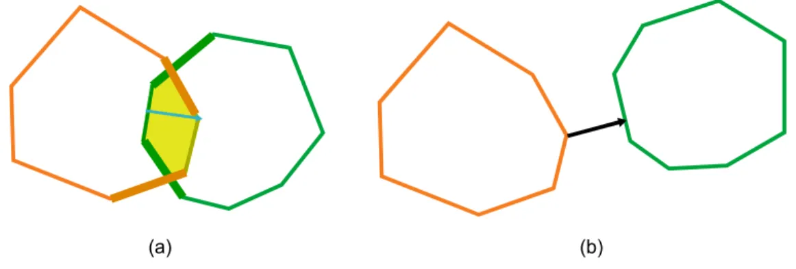
Figure 1.5: Different proximity queries between 2 polygons. (a) The two polygons overlap. The colliding features are shown in bold lines. The penetration depth and direction is given by the blue arrow. (b) The two polygons do not overlap. The separation distance is given by the black arrow.

(32)

The translational penetration depth is defined as the minimum translational distance needed to make the two overlapping objects disjoint [DHKS93]. In this thesis, we shall restrict dis-cussion to translational penetration depth. More recently work has been done in handling rotational penetation depth. Examples of discrete collision, penetration depth and separation distance queries among 2D polygonal objects is provided in figure 1.5.

1.2 Previous Work

There has been extensive study on Voronoi diagrams and medial axis computation in various areas of computer science. This section describes some of the previous work and challenges in computation of the Voronoi diagram of 3D polygonal models. Algorithms for computation of the Voronoi diagram of a general 3D polyhedron are broadly classified into discreteandcontinuousalgorithms.

The discrete algorithms compute an approximation of the Voronoi diagram using a dis-crete sampling of the space. One class of these algorithms approximates the polyhedron by a finite set of point samples on the boundary. There are several efficient and robust algorithms for computing the Delaunay triangulation and Voronoi diagram of a set of points in 3D (see for e.g. [AK00]). However the Voronoi diagram of a set of points in 3D does not converge to the medial axis of the polyhedron. Given a sufficiently dense point sampling of the boundary of a smooth 3D object, practical algorithms have been proposed to compute a subset of the Voronoi diagram of points which converges to its medial axis [ACK01a, DZ02a]. However these approaches can guarantee convergence only for smooth objects - polyhedral models with sharp edges require infinite sampling.

(33)

uniform grids [HCK+99b, FLM03], adaptive grids [VO98, ER02, BCMS05] or unstructured spatial subdivisions [TT97, YBM04, SS06]. Both classes of discrete algorithms compute the Voronoi diagram only to a certain resolution. The exact Voronoi diagram is computed as the underlying sampling approaches infinity. In practice, these algorithms stop at a finite resolu-tion and return an approximate Voronoi diagram. A common deficiency of these methods is that there are no guarantees on the topology of the approximate Voronoi diagram.

Algorithms for accelerating the discrete Voronoi diagram computation on a uniform grid using graphics hardware have been presented [WND97, HCK+99b, Den03b]. The graphics processing unit (GPU) is a programmable parallel vector processors designed for rapid raster-ization of geometric primitives. These approaches present distance field and Voronoi diagram computation as a rasterization problem which can be efficiently performed in parallel on a uniform 2D grid. However the existing algorithms may not be interactive for computations on complex deformable 3D models.

A continuous Voronoi diagram algorithm is independent of the sampling resolution pa-rameter. The continuous approaches for computing the exact Euclidean Voronoi diagram are based ontracingalgorithms [Mil93, SPB96, Cul00]. The tracing algorithm operates on the graph formed by Voronoi edges (seam curves) and Voronoi vertices (junction points) of the 3D Voronoi diagram. The main idea is to construct this graph using breadth-first or depth-first search. The algorithm requires exact computation of intersection points between (non-linear) algebraic curves and ordering of points along an algebraic curve. Thus, the required precision varies as a function of root isolation algorithms and bounds. As a result, continuous methods based on floating-point arithmetic are sensitive to round-off error, while methods based on exact arithmetic are not efficient.

The challenges in computation and application of the Voronoi diagram and medial axis of 3D polyhedral models are as follows:

(34)

diagram is defined as the total number of Voronoi faces (sheets), edges (seams) and vertices (Junctions). Tight bounds on the worst-case complexity of the medial axis are not known. It is currently known to beΩ(n2₎_and_O₍_n3+ǫ₎_{, where}_n_{is the total number of faces, edges and}

vertices on the boundary of the polyhedron. Examples of theΩ(n2₎_{bound are provided by} Culver [Cul00]. The upper bound follows from Sharir and Agarwal [SA95].

In the same work, Sharir and Agarwal present a randomized algorithm for computing the Voronoi diagram in O(n3+ǫ₎ _{time. However, they assume that certain operations, such}

as junction location, take constant time, and this approach may not be suitable for practical implementation. The tracing algorithms have a cost of O(nm), wherem is the complexity of the Voronoi diagram. The cost of the discrete methods depends on the desired resolution and input complexity. For a dense point sampling of a polyhedral surface, the complexity of the Delaunay triangulation is linear in number of points [AB02].

Robust Computation: The accuracy of continuous geometric algorithms depends on the reliable computation of underlying primitives. The two common reliability problems in implementations of geometric algorithms are: failure due to round-off error, and the inabil-ity to handle degenerate configurations. These problems are collectively called robustness problems.

Round-off error is introduced due to finite precision of computer arithmetic. Geometric algorithms are quite sensitive to roundoff error. A small numerical error can lead to incorrect evaluation of a geometric predicate possibly resulting in invalid output.

In addition, often a geometric algorithm assumes, for simplicity, that its input is in gen-eral position. This means that certain rare configurations are disallowed, and an infinitesimal

perturbation of the input usually breaks the configuration. Such a configuration is called a degenerate configuration. This problem is exaggerated by finite-precision arithmetic. In a

(35)

general position. In particular, models of synthetic objects (for e.g. CAD parts) often exhibit symmetry which may lead to degeneracies for geometric algorithms.

One approach for handling robustness problems is to design algorithms which are stable in the presence of round-off error, and insensitive to presence of degeneracies. However, such an approach is rather limited. Many approaches require either a systematic detection of degenerate cases or a systematic way of applying a small perturbation. Such approaches require some form of exact computation.

(a) (b)

Figure 1.6: Near-degenerate configuration of the Voronoi diagram. An almost regular hexagon. The right-most vertex has been perturbed by an infinitesimal amount. (a) The Voronoi diagram of the hexagon (b) Magnified view of the center showing two junctions. Arbitrarily large precision may be required to distinguish the junctions.

Specifically for the continuous algorithms for Voronoi diagram computation, one needs reliable computation of locations of junction points and their ordering on seam curves. This involves solving a system of non-linear tri-variate equations, which reduces to solving equa-tions up-to degree eight. The degenerate cases for Voronoi diagrams of polyhedral models are listed by Culver [Cul00], and some of these cases can be common in solid modeling and processing. An example of a near-degenerate junction is shown in figure 1.6. To detect and correctly handle these degeneracies, Culver uses exact computation, which may not scale efficiently to complex models composed of tens of thousands of polygons.

(36)

This means that small modifications to the boundary of a polyhedron can induce large modi-fications in its Voronoi diagram. A 2D example is shown in figure 1.7. The problem is exag-gerated by the combinatorial complexity of the Voronoi diagram. Noise on the boundary also leads to higher combinatorial complexity. Thus a practical application requires extraction of a stable approximation of the Voronoi diagram or medial axis.

(a) (b)

Figure 1.7: Instability of the medial axis. (a) The medial axis (orange) of a simple polygon. (b) Small perturbation in boundary causes large change in the medial axis.

The stability of the medial axis under small perturbations has been recently studied, and it has been shown that for small perturbation in the boundary of a shape, the original medial axis is contained inside a tight parallel body of the noisy medial axis [ABE04, CS02]. This result provides promise for extraction of a simplified medial axis corresponding to its stable part. The most common approach for medial axis simplification removes parts of the medial axis using a threshold on an importance measure (see [ABE04] for a survey). Typical importance measures used are distance to boundary and the angle subtended by the vectors from a point on the medial axis to its footprints.

(37)

(a) (b) (c)

Figure 1.8:Approximate medial axis computation without topological guarantees.(a) A thin CAD model. (b) Approximate medial axis computed using Voronoi diagram of points. (c) Zoomed view of the computed medial axis highlighting regions where homotopy type is not preserved. (Images courtesy GMSWorks, C-Solutions Inc.)

Application to Proximity Queries: The problem of fast and reliable geometric prox-imity queries has been extensively studied. Despite the vast literature, real-time proxprox-imity queries remain one of the major bottlenecks for interactive deformable simulation [TKH+05, MHTG05]. Many existing methods are based on hierarchical representations and work well for rigid models. Several efficient collision detection algorithms have been proposed for deformable models, but they do not compute separation or penetration distances.

The upper bound on complexity of collision detection and separation distance compu-tation is O(m2₎ _where _m _{is the number of primitives. In practice, only a small subset} of primitive pairs needs to be tested for exact proximity computations. Most prior algo-rithms for proximity queries perform culling tests based on bounding volume hierarchies such as spheres or axis-aligned bounding boxes (AABBs). Tighter bounding volume hierar-chies achieve higher culling at a cost of increased computation time. Thus these algorithms may not work well for dynamic environments involving close proximity scenarios or for intra-object queries. In addition, exact computation of PD between two polyhedral models is a global problem and cannot be solved using any ‘divide-and-conquer’ or localized ap-proach [KOLM02]. Its worst complexity can be as high as O(n3

(38)

External Voronoi regions of convex polytopes have been used to perform collision and distance queries between rigid objects that can be represented as union of convex poly-topes [LC91b, Mir98]. These algorithms have been implemented within different proximity query packages such as I-COLLIDE, V-CLIP and SWIFT++ [Eri04]. However, it is hard to extend these algorithms to general non-convex deformable models. This is due to lack of robust algorithms for computing Voronoi diagrams of polygonal models at interactive rates.

Thus, robust and efficient computation of the Voronoi diagram and medial axis of 3D polyhedral models remains a challenging problem, limits their application.

1.3 Thesis

Our thesis is

The discrete Voronoi diagram and simplified medial axis of 3D polyhedral models can

be computed efficiently with geometric and topological guarantees, and can be used for fast

proximity queries among multiple deformable models.

In this thesis we present efficient algorithms for computing discrete Voronoi diagram and approximate medial axis of complex 3D polyhedral models. We describe an algorithm to compute 3D distance fields of geometric models by using a linear factorization of Euclidean distance vectors. This formulation maps directly to the linearly interpolating graphics ras-terization hardware and enables us to compute distance fields of complex 3D models at in-teractive rates. We also use clamping and culling algorithms based on properties of Voronoi diagrams to accelerate this computation. We provide geometric guarantees on the result using Hausdorff distance bounds.

(39)

deformable models using second order discrete Voronoi diagrams. We show the reduction of different proximity queries to specializations of N-body distance queries. We also present an algorithm to reliably and efficiently compute N-body distance queries using the second order discrete Voronoi diagram.

We also present an adaptive sampling algorithm to provide topological guarantees on the approximate Voronoi diagram. Our algorithm uses subdivision criteria to compute an approximate Voronoi diagram which is homotopy equivalent to the exact Euclidean Voronoi diagram, and can handle degenerate configurations in the input polyhedron. The subdivision criteria is based on computing the arrangement of 2D conic sections, which can be performed accurately and efficiently [Be05, KCMh99]. Finally, we present an algorithm for efficiently computing the homotopy-preserving simplified medial axis from the approximate Voronoi diagram.

1.3.1 New Results

This dissertation presents contributions to interactive computation of discrete Voronoi di-agrams, fast proximity computation among multiple deformable models and efficient compu-tation of a homotopy-preserving Voronoi diagram and simplified medial axis for polyhedral models. The main results are described below.

Interactive computation of Discrete Voronoi Diagrams

(40)

• Computation of Voronoi region bounds. We present a multi-pass algorithm that exploits geometric properties of Voronoi diagrams to compute Voronoi region bounds in 2D and 3D. The underlying approach also extends to higher dimensions.

• Culling techniques for distance computations. We present culling techniques for 3D distance field and discrete Voronoi diagram computation using Voronoi region bounds and coherence of distance fields. The domain is divided into ranges, and sites which do not contribute to the Voronoi diagram within a range are culled away.

• Surface Distance Maps:. We present a new algorithm for computing the distance map and discrete Voronoi diagram on a triangulated mesh. We use simple texture represen-tation to store a piecewise planar parametrization of the mesh. The parameterization defines an affine transformation for each primitive of the mesh. The affine transfor-mation of the geometric primitive is applied to compute the distance functions of 3D primitives using the texture mapping hardware. This representation, called surface distance map, is used to perform efficient and accurate proximity queries.

Fast proximity computation among multiple deformable models

• N-body distance query:We introduce a unified approach to perform different proxim-ity queries usingN-body distance computation: given a set _P of primitives, for each primitive pi we compute the closest primitive in _{P \ {}pi_}. We also present efficient algorithms for continuous collision detection and local penetration depth computation based on the N-body distance query.

(41)

di-agram because it provides information about two closest primitives at each point in space and results in a higher culling efficiency.

• Fast and conservative computations using discrete Voronoi diagrams:The exact com-putation of continuous 3D Voronoi diagrams for general triangulated models is a hard problem. Instead, we compute discrete Voronoi diagrams on a uniform grid using graphics hardware. We exploit properties of the 2nd_{order Voronoi diagram to derive}

distance error bounds that take into account discretization and sampling errors in dis-crete Voronoi diagrams. We use the distance bounds to efficiently compute the closest primitive at object-space precision i.e. IEEE64-bit floating point accuracy.

Computation of homotopy-preserving simplified medial axis

• Topological properties: We present an algorithm to compute an approximate Voronoi diagram that is homotopy equivalent to the exact Voronoi diagram. To provide this guarantee we exploit topological properties of the Voronoi diagram of a polyhedral model, and use a subdivision scheme based on accurate 2D tests.

• Computing arrangement of 2D conic sections: The topological tests used in the sub-division scheme reduce to computing an arrangement of 2D conic sections on a plane, instead of computing an arrangement of 3D quadric surfaces. The arrangement of 2D conics has been well studied and good implementations are available. As a result, this algorithm is relatively simple to implement as compared to exact 3D Voronoi diagram computation algorithms and does not require arbitarily high precision to compute the junctions.

(42)

• Computing stability of medial axis parts: We present a relationship between the stabil-ity of medial axis junctions and seams to stabilstabil-ity of incident sheets using separation angles. We also present an algorithm to compute a bounded approximation of this stability measure using discrete sampling.

As compared to prior approaches, the algorithms presented in this thesis have several advantages:

• Generality: The distance field and discrete Voronoi diagram computation algorithms make no assumptions with regards to the input models. The objects can have complex topologies, may be non-orientable or non-manifold surfaces, or may be represented using voxel data.

• Non-rigid Motion: The algorithms involve no precomputation and are directly appli-cable to dynamic models undergoing non-rigid motion, and changing topologies.

• Efficiency: Discrete Voronoi diagram and proximity computation are up-to an order of magnitude faster than prior approaches, with improved culling efficiency and tighter bounds. As a result, we achieve interactive performance for complex models consisting of thousands of primitives.

• Accuracy: Discrete Voronoi diagram computation on the GPU is performed at 32-bit floating point precision. In addition, tight geometric bounds are provided on the accuracy of the discrete Voronoi diagram. In addition, the algorithms are designed to account for under-sampling errors due to limited frame buffer precision on the GPU.

(43)

1.3.2 Organization

(44)

(45)

Chapter 2 Fast 3D Discrete Voronoi Diagram

Computation

Many algorithms have been proposed to compute discretized Voronoi diagrams and dis-tance fields along uniform grids using graphics rasterization hardware [WND97, HCK+99b, SPG03]. Graphics processing units (GPUs) are programmable vector processors designed for rapid rasterization of geometric primitives. Moreover, GPUs have been growing at a rate faster than the Moore’s Law over the last decade, making them attractive for certain general purpose parallel computations.

These existing algorithms rasterize the distance functions of the geometric primitives and use the depth buffer hardware to compute an approximation of the lower envelope of the distance functions. The algorithms for general polygonal primitives approximate the non-linear distance functions using a distance mesh. This can be expensive for complex models and the accuracy of the overall approach is governed by the tessellation error. As a result, previous techniques are unable to compute 3D distance fields of complex models at interactive rates.

(46)

a brief overview of general purpose computation capabilities of current graphics hardware. We then present linear factorization of Euclidean distance vectors. This formulation maps di-rectly to the linearly interpolating graphics rasterization hardware and enables us to compute distance fields of complex 3D models at interactive rates. We also use clamping and culling algorithms based on properties of Voronoi diagrams to accelerate this computation.

2.1 Previous Work

In this section we give a brief overview of previous work on computing discrete Voronoi diagrams and distance fields. We also mention some GPU-based algorithms to evaluate non-linear functions.

2.1.1 Distance Fields and Discrete Voronoi Diagrams

The algorithms for distance field and discrete Voronoi diagram computation can be broadly categorized based on different model representations such as images, volumes or polygonal representations.

(47)

propagation front in dynamic lists [Egg98, Rag92]. Propagation methods can be augmented by storing additional information like direction vectors to nearest voxel [Mul92] and closest features [HLC+01]. Propagating additional information along with the FMM, leads to an exact distance transform algorithm [BMW00]. A linear time algorithm for computing ex-act Euclidean distance transform of a2-D binary image is presented in [BGKW95]. This is extended tok-D images and other distance metrics [MQR03].

Geometric Models. There is extensive work in computing the exact Voronoi diagram of a set of points as the dual of the Delaunay triangulation of the points. A good survey of these algorithms is given in [Aur91].

For geometric models represented using polygonal or higher order surfaces in 3D, many algorithms compute an approximation to the Voronoi diagram by computing distance fields on a uniform grid or an adaptive grid. A key issue in generating discrete distance samples is the underlying sampling rate used for adaptive subdivision. Adaptive refinement strate-gies for distance field computation use trilinear interpolation or curvature information to generate an octree spatial decomposition [SFYC96, FPRJ00, PF01]. Although, these al-gorithms optimize the sparsity of the octree representation, the approximation using a tri-linear interpolation may not work well for curved primitives or when the final surface has a lot of sharp features. Adaptive refinement approaches for Voronoi diagram computation use a Voronoi region based labeling of the sample points to generate an spatial decomposi-tion [VO98, TT97, ER02].

(48)

is proposed in [Den03a]. It uses precomputed depth textures, and a quadtree to estimate Voronoi region bounds. However, the extension of this approach to higher dimensions or higher order primitives is not presented. A class of exact distance transform algorithms is based on computing partial Voronoi diagrams [Lin93]. A scan-conversion method to compute the 3-D Euclidean distance field in a narrow band around manifold triangle meshes is the Characteristics/Scan-Conversion (CSC) algorithm [Mau03]. The CSC algorithm uses the connectivity of the mesh to compute polyhedral bounding volumes for the Voronoi cells. The distance function for each site is evaluated only for the voxels lying inside this polyhedral bounding volume. An efficient GPU based implementation of the CSC algorithm is presented in [SPG03]. The number of polygons sent to the graphics pipeline is reduced and the non-linear distance functions are evaluated using fragment programs.

2.1.2 GPU-Based Non-linear Computations

(49)

2.2 Notation and Background

In this section we provide notation used in the chapter and brief overview of graphics processing units (GPUs) with specific details on features useful for interactive distance field computation. We also summarize the existing work on distance field computation using GPUs.

2.2.1 Terminology

Letq= (q1, q2, . . . , qn)denote a point in ndimensions. For points in 3-dimensions, we use the standard Cartesian coordinates,q = (qx, qy, qz). A geometric primitive or an object is called asite. In this work, a site is a vertex, an open edge or an open triangle. Thepivot point of a site is any point lying on the site, and is representedκ(pi). In practice, we use the centroid of a site as its pivot point.

Given a sitepi, the scalar distance function d₍_{q, pi}₎_{denotes the distance from the point} q _∈ _Rn to the closest point on pi. Let _P = {p1, p2, . . . , pm}denote a set of msites. The minimum distance ofqto _P is represented as d₍_q,_P_{) = min}_p

i∈P(d(q, pi)). Thedistance

fieldD_D(P), for a domain_{D ⊂}_R3, is the scalar field given by the minimum distance function

d₍_q,_P₎_{for all points}_q_{∈ D}_{. For ease of notation, let}_D_D ₌_D_D₍_P₎_{. Given a subset,}_{X ⊂ P}_, d₍_q,_X₎_≥d₍_q,_P₎_∀_q_{∈ D}_.

Distance fields are closely related to Voronoi diagrams. The Voronoi region for pi is defined as:

V(i) = {q_|d₍_{q, pi}₎_≤d₍_{q, pj}₎_∀_pj _{∈ P}_,_q_{∈ D}}

The Voronoi diagram is a partition of_DintomVoronoi regions:

VD(P,D) = [

pi,pj∈P,i6=j

(50)

The Voronoi diagram can be represented as the projection of the distance field to the do-main_D[ES86].

Our goal is to compute adiscrete Voronoi diagramwithin a bounded domain_D. Given a finite set of point samples_Dein domain_D, and a set of sites_P, thediscrete Voronoi diagram (DVD) is a partition of the point samples onto discrete Voronoi regions, and is denoted as

g

VD(_P). The discrete Voronoi region is a finite set of points which are closer to one site than to any other site, and is denoted _Ve(pi). We require that the domain _D is a superset of the bounding box of all sites. This assumption is used to guarantee correctness of the culling algorithm. The finite set of point samples_De lie along a uniform grid. Without loss of generality, we can scale the domain_D to be the half-open unit interval in n-dimensions

(0,1]n_{, i.e a unit square in 2D and the unit cube in 3D. To apply our culling algorithm in}

dimensions, we introduce D ranges. We shall refer to an dimensional hypercube as an n-Drange(a rectangular tile in 2D, a cube in 3D). The n-D range(a0, b0]×(a1, b1]×. . .×(an, bn] is represented asT(a0,b0](a1,b1]...(an,bn]. We define each range to be a half-open set such that the

intersection between two ranges is empty, and any point in_Dbelongs to exactly one range. For ease of notation, letVD(_P,_D) = VD(_P). In this chapter, we shall denote the Voronoi diagram computed on a rangeTasVDT(_P). Let_Xc,∂_X andInt(_X)denote the complement, boundary and interior of a set_X, respectively. For any domain N ⊆ D, Nc ₌ _{D \}_N_{. For}

3D grids, the set of cells with a constantz-value represents a uniform 2D grid and is called a slice. A sliceskis defined assk ={(x, y, z)|(x, y, z)∈ D, z =zk}.

2.2.2 Distance Field Computation using GPUs

A brute-force algorithm to computeVD(g _P) would evaluated₍_q₎_pi _{for all sites}_pi _{∈ P}

and store the minimum at each grid pointq _∈ _De. If there arem sites, and the grid hasM

(51)

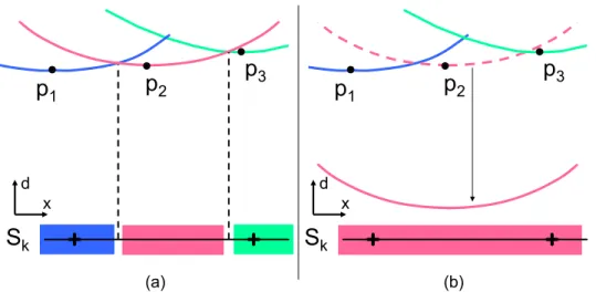
Graph-ics hardware is well suited for performing parallel computations on a 2D grid. Computation of the lower envelope is posed as a visibility problem along a view direction that is orthogo-nal to the 2D grid. The visibility test is efficiently performed using the depth test on graphics hardware. The discrete Voronoi diagram is computed along with the distance field. In 2D, the resolution of the grid is governed by the image-space resolution of the graphics processors (e.g.1000×1000).

(a) (b) (c)

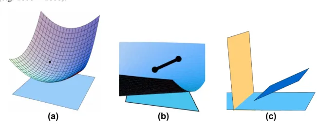
Figure 2.1: Quadratic distance function from a site to a plane: The graph representing the Euclidean distance from a site to a point on a plane is a quadric surface. (a) A paraboloid for a point site (b) An elliptical cone for a line site (c) A pair of planes for a planar polygon.

The 3D distance field is computed by sweeping along the Z axis. For each slice, the distance field is computed using the distance from the sites to the plane [HCK+99b, SPG03]. The underlying distance function is a degree two function (i.e. a quadric surface in 3D). For example, the Euclidean distance function of a point site to a plane is one sheet of the hyperboloid, and of a line to a plane is an elliptical cone, shown in figure 2.1.

(52)

point (or pixel) on the plane. They briefly mention use of bilinear interpolation, and present an approach which uses several instructions per fragment to compute the distance function. However, their approach does not compute the exact discrete Voronoi diagram.

2.3 Linear Factorization

In contrast to earlier approaches, we compute the distance function for each site by eval-uating the distance vector field on the GPU. A distance vector field consists of vectors from the 3D points to the closest point on the site. The magnitude of the distance vector provides the value of the distance function of the site at a grid point. We first present a formulation to compute the distance vector at any point on a planar polygon by using the distance vec-tors of the polygon vertices to the site. Next, we present techniques to compute these planar polygons which bound a site’s Voronoi region on a slice. Finally, we map the problem of distance vector computation to texture mapping hardware on the GPU. Linear factorization

(53)

of distance vectors is used to evaluate the distance functions. Formally speaking, the linear factorization expresses the distance vector at each point inside the polygon in terms of bilin-ear interpolation of the distance vectors of the polygon vertices. Given a convex polygonP

with vertices(v1, . . . , vk), the linear factorization expresses the distance vector at any interior pointpof the polygon as

~

d(p, pi) =

k X

i=1

αi~d(vi, pi),

where

p=

k X

i=

αivi,0≤αi ≤1 and

k X

i=1

αi = 1.

We present three key properties of distance vector computation at a point on a plane to point sites, line segment sites, and triangular sites. These properties are used to evaluate the dis-tance functions efficiently. We first highlight the property to perform linear factorization of the distance vector of a point on a line to a point site.

Property 2.1. Given two pointsaandbon a plane and a point sitep. Letd~aandd~bdenote the distance vectors ofaandb toprespectively. Then, the distance vectord~xof any point

x = αa+ (1₋α)b,0 _≤ α ≤ 1 is the linear combination of distance vectors ofaand b,

andd~x =α ~da+ (1−α)d~b.

Property 2.1 indicates that given the distance vectors of the vertices of any planar primitive to a point site, the distance vector of any interior point can be computed using a bilinear interpolation of the distance vectors of vertices.

The distance vector of a point xthat projects orthogonally to the interior of a line seg-ment is a vector perpendicular to the line. We use the following property to perform linear factorization of the distance vector of a point that projects onto a line segment.

Property 2.2. Given two points aandbon a plane and a line segment lwith end pointse

(54)

respectively. Then, the distance vectord~xof any pointx=αa+ (1−α)b,0≤α≤1is the

linear combination of distance vectors ofaandb, andd~x=α ~da+ (1−α)d~b.

We use property 2.2 to compute the distance vector of any point that projects ontol. This property indicates that given the vertices of a convex polygon whose projection lies withinl, the distance vector of any interior point in the convex polygon is the bilinear interpolation of the distance vectors of the convex polygon vertices tol.

We extend Property 2.1 and Property 2.2 to compute the distance vector of a pointxthat projects interior to a triangular site. It can be seen that the distance vector ofxis the normal to the triangle.

Property 2.3. Given three pointsa,bandcon a plane and a triangular sitetwith vertices

e, f and g. Let d~a = e− a, d~b = f −b and d~c = g− c denote the distance vectors

of a, b and c to the site t respectively. Then, the distance vector d~x of any point x =

α1a+α2b+ (1−α1−α2)b,0≤α1, α2 ≤1is the linear combination of distance vectors

ofa,b, andcandd~x =α1d~a+α2d~b+ (1−α1−α2)d~c.

Property 2.3 indicates that given the vertices of a convex polygon projecting onto t, the distance vector of any interior point is the bilinear interpolation of the distance vectors of the polygon vertices. Furthermore, the distance vectors of the polygon vertices are normal to the triangular site.

Lemma 2.1. There exists a linear factorization to compute the distance vector of any point to a planar site.

(55)

2.4 Domain Computation

In the previous section we showed that the distance vector from a point in the interior of a convex polygon to a site can be expressed as a bilinear interpolant of the distance vectors at the polygon vertices. In this section, we define the convex domain on a slice for which the distance function of a site is computed. We also present an approach to compute conservative bounds on the domain.

The region where the distance function of a site contributes to the distance field is exactly its Voronoi region. However, it is non-trivial to compute the exact Voronoi regions for higher order sites (i.e. lines, polygons) [CKM98]. Moreover, the Voronoi regions are not necessarily convex. Instead of computing the exact Voronoi region, we compute a convex polygonal domainQi,k on the slice sk, which bounds the intersection of the Voronoi region of sitepi

with slicesk.

We present separate algorithms for manifold and non-manifold sites. We first present an algorithm to compute theQi,k for non-manifold sites. Later, we present an improved

algo-rithm for manifold sites that exploits the connectivity to compute tighter convex polygonal domain.

Non-Manifold Siteswe present the algorithm for a triangle and it can be easily extended to a convex polygon. For a triangletj with verticesp1, p2,p3and unit normalnt, consider the three (open) half-spaces given by planes through the three edges and perpendicular to the plane of the triangle. The half-spaces are given asHi = (x₋pi)·ni≥0, i∈ {1,2,3}, where

nisatisfies(pi−pi+1)·ni = 0,nt·ni = 0. Any point in the intersection of these halfspaces is closer to the interior of the triangle, and any point not contained in the intersectionH1∩

H2 ∩H3 is closer to one of the sites on the boundary of the triangle. The convex polygonal domainQj,k is the intersection of the three half-spaces with slicesk.

(56)

p

s

e

H

₁

H

₂

t

s

(c)

(b)

(a)

Figure 2.3: Domain of distance field computation on a slices for non-manifold sites: The domain of computation is shaded in grey. (a) For a point site p, the domain is the entire slice (b) For a line segmente, the domain is bounded by two parallel half-planesH1andH2, perpendicular toe. (c) For a trianglet, the domain is bounded by triangular prism defined by intersection of three half planes perpendicular to triangle edges.

0andH2 = (p1−p2)·(x−p2)>0. Any pointxin the intersection of the two half spaces is closer to the interior of the line segmente,and a point not in the intersection will be closer

to one of the end points. Thus, the convex polygonal domainQj,k is the intersection of the two half spacesH1, H2with the slicesk.

Finally, given a pointpj, the domainQj,k is the entire slicesk.

Manifold SitesFor a manifold site, we exploit the neighborhood information to compute a convex polytopeGiwhich bounds the Voronoi region of a sitepi[Cul00, Mau03, SPG03]. For a particular slicesk, the domain of computation of a sitepi is given by the intersection of the polytope with the slice,Qi,k = Gi _∩sk. For a triangle site, the bounding polytope is given by a triangular prism defined by intersection of three half spaces (as described above). For an edge e incident on two triangles with normalsn1, n2, the convex polytope is a wedge obtained by the intersection of four half-spaces. Two of the half-spaces are defined by parallel planes through the end vertices of the edge as shown above. The other two half-spaces are defined by planes containing the edgee and have normalsn1 andn2.

(57)

the half-space intersection, with time complexityO(nlogn), we present a simple algorithm to compute a conservative approximation of the bounding polytopeGp for a point site pin

O(n)time.

A point site is defined as convex iff all edges incident on the point have an internal dihe-dral angle less thanπ. Letpbe a convex point, with incident edgesei, 1≤ i ≤ n in order.

Then edges of the convex polytopeGp are given byp+λni, whereni =ei×ei+1(modulo

n) andni is the normal of the triangleti containing edgesei andei+1.

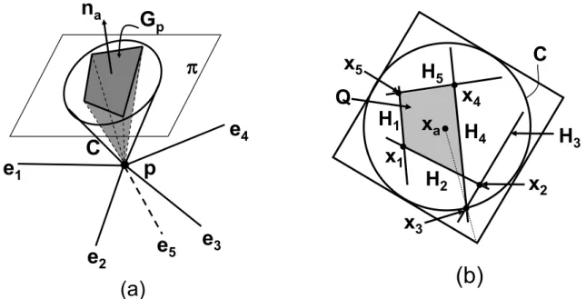
This construction does not work for hyperbolic points[PS05]. Previous approaches ex-pand the bounding polytopes of adjacent triangles to handle hyperbolic points, however this results in a complex fragment program to compute the distance functions [SPG03]. We present an efficient algorithm to compute a bounding polytopeGp for a hyperbolic point p (see figure 2.4(a)). Let na be the average of the normals of all incident triangles. Let nj be the normal which maximizes θ(i) = na×ni

|na×ni|, i = 1, . . . , n. We consider the case when

θ(i) < π/2. LetC be a right circular cone with axisna and opening angle2θ(j). We now prove that the bounding polytopeGpis a subset of coneC.

Theorem 2.1. Letp be a manifold point, andC be a cone constructed as above. Then the convex polytopeGpbounding the Voronoi region ofpis a subset ofC.

Proof. IfGp =∅, then the result trivially holds. It is sufficient to show thatGp∩πk ⊆C∩πk for any plane πk. Consider a plane π orthogonal to na, and let Q be the convex polygon obtained by intersection ofGpwithπ,Q=Gp∩π. Letxibe the intersection of the ray from

palong directionni. Gp∩πis the convex region given by the intersection of 2D half spaces, each half space is given by the line throughxi andxi+1 (modulon) (see figure 2.4(b)). For any pointy _∈ π, let r = maxi=1,...,nd(xi)y. By construction, a circle cwith center yand radiusrwill containQ. Takingy=xa, we getc=C∩πandGp⊆C.

(58)

Figure 2.4: Bounding polytope computation for a hyperbolic point: p is hyperbolic point with5incident edgese_i,i = 1, . . . ,5. (a) The polytopeGp bounds the Voronoi region ofp.

Gpis bounded by a coneC. (b) Intersection ofGpwith planeπ, showing construction ofC.

bounding polytopeGp of a hyperbolic pointp. We use a square pyramid to approximate the bounding polytope as shown in figure. Ifθ(i) _≥ π/2, then we treat the hyperbolic point as non-manifold.

2.5 Distance Field Computation using GPUs

In this section, we present our algorithm for distance computation on the GPU using linear factorization. Given a site and a slice, the convex domain is computed as described in Section 2.4. The distance vector to the site is computed at each vertex of the convex polygon. The distance vector is encoded as a 3D texture coordinate, and the polygon is rasterized on the GPU.

(59)

vectors of the form(vx, vy, vz, vw)and transformations are applied to the attributes in the ver-tex processing unit. The transformed vertices are bilinearly interpolated by the rasterization hardware and the interpolated vectors at each fragment are used for lighting computations using Gouraud or Phong shading, or environment mapping applications. In order to achieve higher performance, the rasterization hardware consists of multiple vector units to compute the interpolated vectors.

We use the fast bilinear interpolation capabilities of GPUs for distance vector computa-tion. Based on the linear factorization formulation, we map the distance vector computation to the GPUs using vertex attributes of the polygons. We use orthographic transformations and perform a one-to-one mapping between the points on the plane and the pixels on the screen. The bilinear interpolation of the vertex attributes is used for distance vector computation at each point on the plane.

The interpolation units in current GPUs can perform computations on different vector representations. For example, the vectors can be represented using 8-bit, 16-bit or 32-bit floating point values and the vector components may be signed or unsigned. Since the com-ponents of the distance vectors are signed and represented in 32-bit floating point precision, we use the 3D texture co-ordinates of the vertices to represent the distance vectors of ver-tices. The interpolated texture co-ordinates are used in a single instruction fragment program to compute the magnitude of the distance vector. The distance field is updated to compute the minimum either using theM IN instruction in the fragment program or by using the depth test functionality.

We now present the expressions for computing the distance vectors from a convex poly-gon vertex to a point, an edge and a triangle. These are:

• Point:Given a point sitepand a vertexv, the distance vector fromvtopis~d(p,v) =

p₋v.

(60)

eis~d(e,v) = (p1−v) +λ(p 2−p1)

|p2−p1|, whereλ=

(v−p1)·(p2−p1) |p2−p1| .

• Triangle: Given a trianglet with a unit normalnˆ, the distance vector from a vertexv

totis given as~d(t,v) = [(pi−v)·nˆ]nˆ, wherepiis one of the three vertices of thet.

The pseudocode for computing the distance field for a sliceskis presented in Algorithm 1. The functionComputePolygon(pi,sk) computes the convex polygonal domain bounding the Voronoi region of sitepi on slicesk.

Input: slicesk, site setP

Output: distance fieldDsk(P)

foreachsitepi ∈ P do 1

Qi,k ←ComputePolygon(pi, sk)

2

foreachvertexv_∈Qi,k do 3

Compute distance vector~d(pi,v)

4

Assign texture coordinates ofv,(r, s, t)←~d(pi,v)

5

end 6

Draw textured polygonQi,k at depthz = 0

7 end 8

Algorithm 1: ComputeSlice(sk,_P): This algorithm computes the distance field for

skfor a set of primitives_P

Efficient computation of discrete Voronoi diagram and homotopy-preserving simplified medial axis of a 3d polyhedron